Reinforcement Learning with Long Short-Term Memory
Reinforcement Learning with Long Short-Term Memory
Reinforcement Learning with Long Short-Term Memory

Create successful ePaper yourself
Turn your PDF publications into a flip-book with our unique Google optimized e-Paper software.
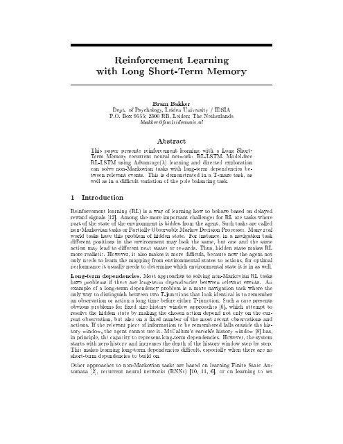
<strong>Reinforcement</strong> <strong>Learning</strong><br />
<strong>with</strong> <strong>Long</strong> <strong>Short</strong>-<strong>Term</strong> <strong>Memory</strong><br />
Bram Bakker<br />
Dept. of Psychology, Leiden University / IDSIA<br />
P.O. Box 9555; 2300 RB, Leiden; The Netherlands<br />
bbakker@fsw.leidenuniv.nl<br />
Abstract<br />
This paper presents reinforcement learning <strong>with</strong> a <strong>Long</strong> <strong>Short</strong>-<br />
<strong>Term</strong> <strong>Memory</strong> recurrent neural network: RL-LSTM. Model-free<br />
RL-LSTM using Advantage() learning and directed exploration<br />
can solve non-Markovian tasks <strong>with</strong> long-term dependencies between<br />
relevant events. This is demonstrated in a T-maze task, as<br />
well as in a dicult variation of the pole balancing task.<br />
1 Introduction<br />
<strong>Reinforcement</strong> learning (RL) is a way of learning how tobehave based on delayed<br />
reward signals [12]. Among the more important challenges for RL are tasks where<br />
part of the state of the environment ishidden from the agent. Such tasks are called<br />
non-Markovian tasks or Partially Observable Markov Decision Processes. Many real<br />
world tasks have this problem of hidden state. For instance, inanavigation task<br />
dierent positions in the environment may look the same, but one and the same<br />
action may lead to dierent next states or rewards. Thus, hidden state makes RL<br />
more realistic. However, it also makes it more dicult, because now the agent not<br />
only needs to learn the mapping from environmental states to actions, for optimal<br />
performance it usually needs to determine which environmental state it is in as well.<br />
<strong>Long</strong>-term dependencies. Most approaches to solving non-Markovian RL tasks<br />
have problems if there are long-term dependencies between relevant events. An<br />
example of a long-term dependency problem is a maze navigation task where the<br />
only way to distinguish between two T-junctions that look identical is to remember<br />
an observation or action a long time before either T-junction. Such a case presents<br />
obvious problems for xed size history window approaches [6], which attempt to<br />
resolve the hidden state by making the chosen action depend not only on the current<br />
observation, but also on a xed number of the most recent observations and<br />
actions. If the relevant piece of information to be remembered falls outside the history<br />
window, the agent cannot use it. McCallum's variable history window [8] has,<br />
in principle, the capacity to represent long-term dependencies. However, the system<br />
starts <strong>with</strong> zero history and increases the depth of the history window step by step.<br />
This makes learning long-term dependencies dicult, especially when there are no<br />
short-term dependencies to build on.<br />
Other approaches to non-Markovian tasks are based on learning Finite State Automata<br />
[2], recurrent neural networks (RNNs) [10, 11, 6], or on learning to set
memory bits [9]. Unlike history window approaches, they do not have to represent<br />
(possibly long) entire histories, but can in principle extract and represent just the<br />
relevant information for an arbitrary amount of time. However, learning to do that<br />
has proven dicult. The diculty lies in discovering the correlation between a<br />
piece of information and the moment atwhich this information becomes relevant<br />
at a later time, given the distracting observations and actions between them. This<br />
diculty can be viewed as an instance of the general problem of learning long-term<br />
dependencies in timeseries data. This paper uses one particular solution to this<br />
problem that has worked well in supervised timeseries learning tasks: <strong>Long</strong> <strong>Short</strong>-<br />
<strong>Term</strong> <strong>Memory</strong> (LSTM) [5, 3]. In this paper an LSTM recurrent neural network is<br />
used in conjunction <strong>with</strong> model-free RL, in the same spirit as the model-free RNN<br />
approaches of [10, 6]. The next section describes LSTM. Section 3 presents LSTM's<br />
combination <strong>with</strong> reinforcement learning in a system called RL-LSTM. Section 4<br />
contains simulation results on non-Markovian RL tasks <strong>with</strong> long-term dependencies.<br />
Section 5, nally, presents the general conclusions.<br />
2 LSTM<br />
LSTM is a recently proposed recurrent neural network architecture, originally designed<br />
for supervised timeseries learning [5, 3]. It is based on an analysis of the<br />
problems that conventional recurrent neural network learning algorithms, e.g. backpropagation<br />
through time (BPTT) and real-time recurrent learning (RTRL), have<br />
when learning timeseries <strong>with</strong> long-term dependencies. These problems boil down<br />
to the problem that errors propagated back in time tend to either vanish or blow<br />
up (see [5]).<br />
<strong>Memory</strong> cells. LSTM's solution to this problem is to enforce constant error ow<br />
in a number of specialized units, called Constant Error Carrousels (CECs). This<br />
actually corresponds to these CECs having linear activation functions which do<br />
not decay over time. In order to prevent the CECs from lling up <strong>with</strong> useless<br />
information from the timeseries, access to them is regulated using other specialized,<br />
multiplicative units, called input gates. Like the CECs, the input gates receive input<br />
from the timeseries and the other units in the network, and they learn to open and<br />
close access to the CECs at appropriate moments. Access from the activations of<br />
the CECs to the output units (and possibly other units) of the network is regulated<br />
using multiplicative output gates. Similar to the input gates, the output gates learn<br />
when the time is right to send the information stored in the CECs to the output<br />
side of the network. A recent addition is forget gates [3], which learn to reset<br />
the activation of the CECs when the information stored in the CECs is no longer<br />
useful. The combination of a CEC <strong>with</strong> its associated input, output, and forget<br />
gate is called a memory cell. See gure 1b for a schematic of a memory cell. It is<br />
also possible for multiple CECs to be combined <strong>with</strong> only one input, output, and<br />
forget gate, in a so-called memory block.<br />
Activation updates. More formally, the network's activations at each timestep<br />
t are computed as follows. A standard hidden unit's activation y h , output unit<br />
activation y k , input gate activation y in , output gate activation y out , and forget<br />
gate activation y ' is computed in the following standard way:<br />
y i (t) =f i ( X m<br />
w im y m (t , 1)) (1)<br />
where w im is the weight of the connection from unit m to unit i. In this paper, f i<br />
is the standard logistic sigmoid function for all units except output units, for which<br />
it is the identity function. The CEC activation s c v<br />
j<br />
, or the \state" of memory cell v
A a1<br />
A a2<br />
cell output<br />
output gate<br />
hidden<br />
hidden<br />
memory cells<br />
CEC<br />
input gate<br />
forget gate<br />
observation<br />
a. b.<br />
cell input<br />
memory cell<br />
Figure 1: a. The general LSTM architecture used in this paper. Arrows indicate<br />
unidirectional, fully connected weights. The network's output units directly code<br />
for the Advantages of dierent actions. b. One memory cell.<br />
in memory block j, is computed as follows:<br />
s c v<br />
j<br />
(t) =y 'j (t)s c v<br />
j<br />
(t , 1) + y inj (t)g( X m<br />
w c v<br />
j<br />
my m (t , 1)) (2)<br />
where g is a logistic sigmoid function scaled to the range [,2; 2], and s c v<br />
j<br />
(0) = 0.<br />
The memory cell's output y cv j<br />
is calculated by<br />
y cv j (t) =y outj (t)h(s c v<br />
j<br />
(t)) (3)<br />
where h is a logistic sigmoid function scaled to the range [,1; 1].<br />
<strong>Learning</strong>. At some or all timesteps of the timeseries, the output units of the<br />
network may make prediction errors. Errors are propagated just one step back in<br />
time through all units other than the CECs, including the gates. However, errors<br />
are backpropagated through the CECs for an indenite amount of time, using an<br />
ecient variation of RTRL [5, 3]. Weight updates are done at every timestep, which<br />
ts in nicely <strong>with</strong> the philosophy of online RL. The learning algorithm is adapted<br />
slightly for RL, as explained in the next section.<br />
3 RL-LSTM<br />
RNNs, such as LSTM, can be applied to RL tasks in various ways. One way is<br />
to let the RNN learn a model of the environment, which learns to predict observations<br />
and rewards, and in this way learns to infer the environmental state at<br />
each point [6,11]. LSTM's architecture would allow the predictions to depend on<br />
information from long ago. The model-based system could then learn the mapping<br />
from (inferred) environmental states to actions as in the Markovian case, using<br />
standard techniques such as Q-learning [6, 2], or by backpropagating through the<br />
frozen model to the controller [11]. An alternative, model-free approach, and the<br />
one used here, is to use the RNN to directly approximate the value function of a<br />
reinforcement learning algorithm [10, 6]. The state of the environment is approximated<br />
by the current observation, which is the input to the network, together <strong>with</strong><br />
the recurrent activations in the network, which represent the agent's history. One<br />
possible advantage of such a model-free approach over a model-based approach is<br />
that the system may learn to only resolve hidden state insofar as that is useful for<br />
obtaining higher rewards, rather than waste time and resources in trying to predict<br />
features of the environment that are irrelevant for obtaining rewards [6, 8].<br />
Advantage learning. In this paper, the RL-LSTM network approximates the<br />
value function of Advantage learning [4], which was designed as an improvement on
Q-learning for continuous-time RL. In continuous-time RL, values of adjacent states,<br />
and therefore optimal Q-values of dierent actions in a given state, typically dier by<br />
only small amounts, which can easily get lost in noise. Advantage learning remedies<br />
this problem by articially decreasing the values of suboptimal actions in each state.<br />
Here Advantage learning is used for both continuous-time and discrete-time RL.<br />
Note that the same problem of small dierences between values of adjacent states<br />
applies to any RL problem <strong>with</strong> long paths to rewards. And to demonstrate RL-<br />
LSTM's potential to bridge long time lags, we need to consider such RL problems.<br />
In general, Advantage learning may be more suitable for non-Markovian tasks than<br />
Q-learning, because it seems less sensitive to getting the value estimations exactly<br />
right.<br />
The LSTM network's output units directly code for the Advantage values of dierent<br />
actions. Figure 1a shows the general network architecture used in this paper. As<br />
in Q-learning <strong>with</strong> a function approximator, the temporal dierence error E TD (t),<br />
derived from the equivalent of the Bellman equation for Advantage learning [4], is<br />
taken as the function approximator's prediction error at timestep t:<br />
E TD r(t)+V (s(t + 1)) , V (s(t))<br />
(t) =V (s(t)) + , A(s(t);a(t)) (4)<br />
<br />
where A(s; a) is the Advantage value of action a in state s, r is the immediate<br />
reward, and V (s) = max a A(s; a) is the value of the state s. is a discount factor<br />
in the range [0; 1], and is a constant scaling the dierence between values of<br />
optimal and suboptimal actions. Output units associated <strong>with</strong> other actions than<br />
the executed one do not receive error signals.<br />
Eligibility traces. In this work, Advantage learning is extended <strong>with</strong> eligibility<br />
traces, which have often been found to improve learning in RL, especially in<br />
non-Markovian domains [7]. This yields Advantage() learning, and the necessary<br />
computations turn out virtually the same as in Q()-learning [1]. It requires the<br />
storage of one eligibility trace e im per weight w im . Aweight update corresponds to<br />
w im (t+1) = w im (t)+E TD (t)e im (t) , where e im (t) =e im (t ,1)+ @yK (t)<br />
@w im<br />
: (5)<br />
K indicates the output unit associated <strong>with</strong> the executed action, is a learning rate<br />
parameter, and is a parameter determining how fast the eligibility trace decays.<br />
e im (0) = 0, and e im (t , 1) is set to 0 if an exploratory action is taken.<br />
Exploration. Non-Markovian RL requires extra attention to the issue of exploration<br />
[2, 8]. Undirected exploration attempts to try out actions in the same way in<br />
eachenvironmental state. However, in non-Markovian tasks, the agent initially does<br />
not know which environmental state it is in. Part of the exploration must be aimed<br />
at discovering the environmental state structure. Furthermore, in many cases, the<br />
non-Markovian environment will provide unambiguous observations indicating the<br />
state in some parts, while providing ambiguous observations (hidden state) in other<br />
parts. In general, we want more exploration in the ambiguous parts.<br />
This paper employs a directed exploration technique based on these ideas. A separate<br />
multilayer feedforward neural network, <strong>with</strong> the same input as the LSTM<br />
network (representing the current observation) and one output unit y v , is trained<br />
concurrently <strong>with</strong> the LSTM network. It is trained, using standard backpropagation,<br />
to predict the absolute value of the current temporal dierence error E TD (t)<br />
as dened by eq. 4, plus its own discounted prediction at the next timestep:<br />
y v d(t) =jE TD (t)j + y v (t +1) (6)<br />
where y v d (t) is the desired value for output yv (t), and is a discount parameter<br />
in the range [0; 1]. This amounts to attempting to identify which observations are
X<br />
S<br />
G<br />
Figure 2: <strong>Long</strong>-term dependency T-maze <strong>with</strong> length of corridor N = 10. At the<br />
starting position S the agent's observation indicates where the goal position G is in<br />
this episode.<br />
\problematic", in the sense that they are associated <strong>with</strong> large errors in the current<br />
value estimation (the rst term), or precede situations <strong>with</strong> large such errors (the<br />
second term). y v (t) is linearly scaled and used as the temperature of a Boltzmann<br />
action selection rule [12]. The net result is much exploration when, for the current<br />
observation, dierences between estimated Advantage values are small (the standard<br />
eect of Boltzmann exploration), or when there is much \uncertainty" about current<br />
Advantage values or Advantage values in the near future (the eect of this directed<br />
exploration scheme). This exploration technique has obvious similarities <strong>with</strong> the<br />
statistically more rigorous technique of Interval Estimation (see [12]), as well as<br />
<strong>with</strong> certain model-based approaches where exploration is greater when there is<br />
more uncertainty in the predictions of a model [11].<br />
4 Test problems<br />
<strong>Long</strong>-term dependency T-maze. The rst test problem is a non-Markovian<br />
grid-based T-maze (see gure 2). It was designed to test RL-LSTM's capability to<br />
bridge long time lags, <strong>with</strong>out confounding the results by making the control task<br />
dicult in other ways. The agent has four possible actions: move North, East,<br />
South, or West. The agent must learn to move from the starting position at the<br />
beginning of the corridor to the T-junction. There it must move either North or<br />
South to a changing goal position, which it cannot see. However, the location of<br />
the goal depends on a \road sign" the agent has seen at the starting position. If<br />
the agent takes the correct action at the T-junction, it receives a reward of 4. If it<br />
takes the wrong action, it receives a reward of ,:1. In both cases, the episode ends<br />
and a new episode starts, <strong>with</strong> the new goal position set randomly either North or<br />
South. During the episode, the agent receives a reward of ,:1 when it stands still.<br />
At the starting position, the observation is either 011 or 110, in the corridor the<br />
observation is 101, and at the T-junction the observation is 010. The length of the<br />
corridor N was systematically varied from 5 to 70. In each condition, 10 runs were<br />
performed.<br />
If the agent takes only optimal actions to the T-junction, it must remember the<br />
observation from the starting position for N timesteps to determine the optimal<br />
action at the T-junction. Note that the agent is not aided by experiences in which<br />
there are shorter time lag dependencies. In fact, the opposite is true. Initially, it<br />
takes many more actions until even the T-junction is reached, and the experienced<br />
history is very variable from episode to episode. The agent must rst learn to<br />
reliably move to the T-junction. Once this is accomplished, the agent will begin to<br />
experience more or less consistent and shortest possible histories of observations and<br />
actions, from which it can learn to extract the relevant piece of information. The<br />
directed exploration mechanism is crucial in this regard: it learns to set exploration<br />
low in the corridor and high at the T-junction.<br />
The LSTM network had 3 input units, 12 standard hidden units, 3 memory cells, and<br />
= :0002. The following parameter values were used in all conditions: = :98, =<br />
:8, = :1. An empirical comparison was made <strong>with</strong> two alternative systems that<br />
have been used in non-Markovian tasks. The long-term dependency nature of the
Number of successful runs<br />
10<br />
8<br />
6<br />
4<br />
2<br />
0<br />
LSTM<br />
Elman−BPTT<br />
<strong>Memory</strong> bits<br />
5 10 15 20 25 30 40 50 60 70<br />
N: length of corridor<br />
Average number of iterations<br />
1.5<br />
1<br />
0.5<br />
0<br />
2 x LSTM<br />
BPTT<br />
<strong>Memory</strong> bits<br />
5 10 15 20 25 30 40 50 60 70<br />
107<br />
N: length of corridor<br />
Figure 3: Results in noise-free T-maze task. Left: Number of successful runs (out of<br />
10) as a function of N, length of the corridor. Right: Average number of timesteps<br />
until success as a function of N.<br />
15 x 106 N: length of corridor<br />
Number of successful runs<br />
10<br />
8<br />
6<br />
4<br />
2<br />
0<br />
LSTM<br />
Elman−BPTT<br />
<strong>Memory</strong> bits<br />
5 10 15 20 25 30 40 50 60 70<br />
N: length of corridor<br />
Average number of iterations<br />
10<br />
5<br />
0<br />
LSTM<br />
BPTT<br />
<strong>Memory</strong> bits<br />
5 10 15 20 25 30 40 50 60 70<br />
Figure 4: Results in noisy T-maze task. Left: Number of successful runs (out of<br />
10) as a function of N, length of the corridor. Right: Average number of timesteps<br />
until success as a function of N.<br />
task virtually rules out history window approaches. Instead, two alternative systems<br />
were used that, like LSTM, are capable in principle of representing information for<br />
arbitrary long time lags. In the rst alternative, the LSTM network was replaced by<br />
an Elman-style Simple Recurrent Network, trained using BPTT [6]. Note that the<br />
unfolding of the RNN necessary for BPTT means that this is no longer truly online<br />
RL. The Elman network had 16 hidden units and 16 context units, and = :001.<br />
The second alternative is a table-based system extended <strong>with</strong> memory bits that are<br />
part of the observation, and that the controller can switch on and o [9]. Because<br />
the task requires the agent to remember just one bit of information, this system<br />
had one memory bit, and = :01. In order to determine the specic contribution of<br />
LSTM to performance, in both alternatives all elements of the overall system except<br />
LSTM (i.e. Advantage() learning, directed exploration) were left unchanged.<br />
A run was considered a success if the agent learned to take the correct action at the<br />
T-junction in over 80% of cases, using its stochastic action selection mechanism. In<br />
practice, this corresponds to 100% correct action choices at the T-junction using<br />
greedy action selection, as well as optimal or near-optimal action choices leading<br />
to the T-junction. Figure 3 shows the number of successful runs (out of 10) as a<br />
function of the length of the corridor N, for each of the three methods. It also<br />
shows the average number of timesteps needed to reach success. It is apparent that<br />
RL-LSTM is able to deal <strong>with</strong> much longer time lags than the two alternatives. RL-<br />
LSTM has perfect performance up to N = 50, after which performance gradually<br />
decreases. In those cases where the alternatives also reach success, RL-LSTM also<br />
learns faster. The reason why the memory bits system performs worst is probably<br />
that, in contrast <strong>with</strong> the other two, it does not explicitly compute the gradient<br />
of performance <strong>with</strong> respect to past events. This should make credit assignment
less directed and therefore less eective. The Elman-BPTT system does compute<br />
such a gradient, but in contrast to LSTM, the gradient information tends to vanish<br />
quickly <strong>with</strong> longer time lags (as explained in section 2).<br />
T-maze <strong>with</strong> noise. It is one thing to learn long-term dependencies in a noise-free<br />
task, it is quite another thing to do so in the presence of severe noise. To investigate<br />
this, a very noisy variation of the T-maze task described above was designed. Now<br />
the observation in the corridor is a0b, where a and b are independent, uniformly<br />
distributed random values in the range [0; 1], generate online. All other aspects of<br />
the task remain the same as above. Both the LSTM and the Elman-BPTT system<br />
were also left unchanged. To allow for a fair comparison, the table-based memory<br />
bit system's observation was computed using Michie and Chambers's BOXES state<br />
aggregation mechanism (see [12]), partitioning each input dimension into three equal<br />
regions.<br />
Figure 4 shows the results. The memory bit system suers most from the noise.<br />
This is not very surprising because a table-based system, even if augmented <strong>with</strong><br />
BOXES state aggregation, does not give very sophisticated generalization. The two<br />
RNN approaches are hardly aected by the severe noise in the observations. Most<br />
importantly, RL-LSTM again signicantly outperforms the others, both in terms of<br />
the maximum time lag it can deal <strong>with</strong>, and in terms of the number of timesteps<br />
needed to learn the task.<br />
Multi-mode pole balancing. The third test problem is less articial than the<br />
T-mazes and has more complicated dynamics. It consists of a dicult variation of<br />
the classical pole balancing task. In the pole balancing task, an agent must balance<br />
an inherently unstable pole, hinged to the top of a wheeled cart that travels along a<br />
track, by applying left and right forces to the cart. Even in the Markovian version,<br />
the task requires fairly precise control to solve it.<br />
The version used in this experiment is made more dicult by two sources of hidden<br />
state. First, as in [6], the agent cannot observe the state information corresponding<br />
to the cart velocity and pole angular velocity. It has to learn to approximate this<br />
(continuous) information using its recurrent connections in order to solve the task.<br />
Second, the agent must learn to operate in two dierent modes. In mode A, action<br />
1 is left push and action 2 is right push. In mode B, this is reversed: action 1 is right<br />
push and action 2 is left push. Modes are randomly set at the beginning of each<br />
episode. The information which mode the agent is operating in is provided to the<br />
agent only for the rst second of the episode. After that, the corresponding input<br />
unit is set to zero and the agent must remember which modeit is in. Obviously,<br />
failing to remember the mode leads to very poor performance. The only reward<br />
signal is ,1 ifthe pole falls past 12 or if the cart hits either end of the track.<br />
Note that the agent must learn to remember the (discrete) mode information for an<br />
innite amount of time if it is to learn to balance the pole indenitely. This rules<br />
out history window approaches altogether. However, in contrast <strong>with</strong> the T-mazes,<br />
the system now has the benet of starting <strong>with</strong> relatively short time lags.<br />
The LSTM network had 2 output units, 14 standard hidden units, and 6 memory<br />
cells. It has 3 input units: one each for cart position and pole angle; and one for the<br />
mode of operation, set to zero after one second of simulated time (50 timesteps).<br />
= :95, = :6, = :2, = :002. In this problem, directed exploration was<br />
not necessary, because in contrast to the T-mazes, imperfect policies lead to many<br />
dierent experiences <strong>with</strong> reward signals, and there is hidden state everywhere in<br />
the environment. For a continuous problem like this, a table-based memory bit<br />
system is not suited very well, so a comparison was only made <strong>with</strong> the Elman-<br />
BPTT system, which had 16 hidden and context units and = :002.
The Elman-BPTT system never reached satisfactory solutions in 10 runs. It only<br />
learned to balance the pole for the rst 50 timesteps, when the mode information<br />
is available, thus failing to learn the long-term dependency. However, RL-LSTM<br />
learned optimal performance in 2 out of 10 runs (after an average of 6,250,000<br />
timesteps of learning). After learning, these two agents were able to balance the pole<br />
indenitely in both modes of operation. In the other 8 runs, the agents still learned<br />
to balance the pole in both modes for hundreds or even thousands of timesteps<br />
(after an average of 8,095,000 timesteps of learning), thus showing that the mode<br />
information was remembered for long time lags. In most cases, such an agent<br />
learns optimal performance for one mode, while achieving good but suboptimal<br />
performance in the other.<br />
5 Conclusions<br />
The results presented in this paper suggest that reinforcement learning <strong>with</strong> <strong>Long</strong><br />
<strong>Short</strong>-<strong>Term</strong> <strong>Memory</strong> (RL-LSTM) is a promising approach to solving non-Markovian<br />
RL tasks <strong>with</strong> long-term dependencies. This was demonstrated in a T-maze task<br />
<strong>with</strong> minimal time lag dependencies of up to 70 timesteps, as well as in a non-<br />
Markovian version of pole balancing where optimal performance requires remembering<br />
information indenitely. RL-LSTM's main power is derived from LSTM's<br />
property of constant error ow, but for good performance in RL tasks, the combination<br />
<strong>with</strong> Advantage() learning and directed exploration was crucial.<br />
Acknowledgments<br />
The author wishes to thank Edwin de Jong, Michiel de Jong, Gwendid van der Voort<br />
van der Kleij, Patrick Hudson, Felix Gers, and Jurgen Schmidhuber for valuable<br />
comments.<br />
References<br />
[1] B. Bakker. <strong>Reinforcement</strong> learning <strong>with</strong> LSTM in non-Markovian tasks <strong>with</strong> longterm<br />
dependencies. Technical report, Dept. of Psychology, Leiden University, 2001.<br />
[2] L. Chrisman. <strong>Reinforcement</strong> learning <strong>with</strong> perceptual aliasing: The perceptual distinctions<br />
approach. In Proc. of the 10th National Conf. on AI. AAAI Press, 1992.<br />
[3] F. Gers, J. Schmidhuber, and F. Cummins. <strong>Learning</strong> to forget: Continual prediction<br />
<strong>with</strong> LSTM. Neural Computation, 12 (10):2451{2471, 2000.<br />
[4] M. E. Harmon and L. C. Baird. Multi-player residual advantage learning <strong>with</strong> general<br />
function approximation. Technical report, Wright-Patterson Air Force Base, 1996.<br />
[5] S. Hochreiter and J. Schmidhuber. <strong>Long</strong> short-term memory. Neural Computation, 9<br />
(8):1735{1780, 1997.<br />
[6] L.-J. Lin and T. Mitchell. <strong>Reinforcement</strong> learning <strong>with</strong> hidden states. In Proc. of the<br />
2nd Int. Conf. on Simulation of Adaptive Behavior. MIT Press, 1993.<br />
[7] J. Loch and S. Singh. Using eligibility traces to nd the best memoryless policy in<br />
Partially Observable Markov Decision Processes. In Proc. of ICML'98, 1998.<br />
[8] R. A. McCallum. <strong>Learning</strong> to use selective attention and short-term memory in<br />
sequential tasks. In Proc. 4th Int. Conf. on Simulation of Adaptive Behavior, 1996.<br />
[9] L. Peshkin, N. Meuleau, and L. P. Kaelbling. <strong>Learning</strong> policies <strong>with</strong> external memory.<br />
In Proc. of the 16th Int. Conf. on Machine <strong>Learning</strong>, 1999.<br />
[10] J. Schmidhuber. Networks adjusting networks. In Proc. of Distributed Adaptive Neural<br />
Information Processing, St. Augustin, 1990.<br />
[11] J. Schmidhuber. Curious model-building control systems. In Proc. of IJCNN'91,<br />
volume 2, pages 1458{1463, Singapore, 1991.<br />
[12] R. S. Sutton and A. G. Barto. <strong>Reinforcement</strong> learning: An introduction. MIT Press,<br />
Cambridge, MA, 1998.