Advanced Statistical Mechanics Phys. 705 Take-Home Final Exam
Advanced Statistical Mechanics Phys. 705 Take-Home Final Exam
Advanced Statistical Mechanics Phys. 705 Take-Home Final Exam

You also want an ePaper? Increase the reach of your titles
YUMPU automatically turns print PDFs into web optimized ePapers that Google loves.
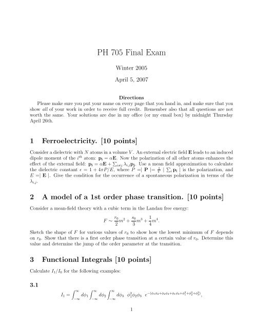
PH <strong>705</strong> <strong>Final</strong> <strong>Exam</strong><br />
Winter 2005<br />
April 5, 2007<br />
Directions<br />
Please make sure you put your name on every page that you hand in, and make sure that you<br />
show all of your work in order to receive full credit. Remember also that all questions are not<br />
worth the same. Your solutions are due in my office (or my email box) by midnight Thursday<br />
April 26th.<br />
1 Ferroelectricity. [10 points]<br />
Consider a dielectric with N atoms in a volume V . An external electric field E leads to an induced<br />
dipole moment of the i th atom: p i = αE. Now the polarization of all other atoms enhances the<br />
effect of the external field: p i = αE + ∑ i≠j λ i,j p j . Use a mean field approximation to calculate<br />
the dielectric constant ǫ = 1 + 4πP/E, where P =| P |= 1 V | ∑ i p i | is the polarization, and<br />
E =| E |. Give the condition for the occurrence of a spontaneous polarization in terms of the<br />
λ i,j .<br />
2 A model of a 1st order phase transition. [10 points]<br />
Consider a mean-field theory with a cubic term in the Landau free energy:<br />
F ∼ r 0<br />
2 m2 + s 0<br />
3 m3 + 1 4 m4 .<br />
Sketch the shape of F for various values of r 0 to show how the lowest minimum of F depends<br />
on r 0 . Show that there is a first order phase transition at a certain value of r 0 . Determine this<br />
value and determine the jump of the order parameter at the transition.<br />
3 Functional Integrals [10 points]<br />
Calculate I 1 /I 0 for the following examples:<br />
3.1<br />
I 1 =<br />
∫ ∞<br />
−∞<br />
dφ 1<br />
∫ ∞<br />
−∞<br />
dφ 2<br />
∫ ∞<br />
−∞<br />
dφ 3 φ 2 1 φ 2φ 3 e −(φ 1φ 2 +φ 2 φ 3 +φ 1 φ 3 +φ 2 1 +φ2 2 +φ2 3 ) ,<br />
1
PH <strong>705</strong> <strong>Final</strong> <strong>Exam</strong>, Winter 2005 2<br />
I 0 =<br />
∫ ∞<br />
−∞<br />
dφ 1<br />
∫ ∞<br />
−∞<br />
dφ 2<br />
∫ ∞<br />
−∞<br />
dφ 3 e −(φ 1φ 2 +φ 2 φ 3 +φ 1 φ 3 +φ 2 1 +φ2 2 +φ2 3 ) .<br />
3.2<br />
I 1 =<br />
∫ ∞<br />
I 0 =<br />
−∞<br />
∫ ∞<br />
dφ 1<br />
∫ ∞<br />
−∞<br />
−∞<br />
dφ 1<br />
∫ ∞<br />
dφ 2<br />
∫ ∞<br />
−∞<br />
−∞<br />
dφ 2<br />
∫ ∞<br />
dφ 3<br />
∫ ∞<br />
−∞<br />
−∞<br />
dφ 3<br />
∫ ∞<br />
dφ 4 φ 1 φ 4 e −[φ 1φ 2 +φ 2 φ 3 +φ 3 φ 4 +φ 1 φ 4 + 3 2 (φ2 1 +φ2 2 +φ2 3 +φ2 4 )] ,<br />
−∞<br />
dφ 4 e −[φ 1φ 2 +φ 2 φ 3 +φ 3 φ 4 +φ 1 φ 4 + 3 2 (φ2 1 +φ2 2 +φ2 3 +φ2 4 )] .<br />
4 Gaussian approximation with an external field. [15<br />
points]<br />
Calculate the longitudinal and transverse correlation functions for T
PH <strong>705</strong> <strong>Final</strong> <strong>Exam</strong>, Winter 2005 3<br />
7 One dimensional Ising model [15 points]<br />
Consider a 1-D Ising model with N particles in an external field h:<br />
N∑<br />
N∑<br />
H(σ 1 , ..., σ n ) = −TK σ i σ i+1 − TH σ i ,<br />
i=1<br />
i=1<br />
with σ i = ±1, and H = h/T, and cyclic boundary conditions: σ N+1 = σ 1 .<br />
7.1<br />
Show that the partition function Z N can be written as<br />
Z N = ∑ σ 1<br />
... ∑ σ N<br />
V σ1 ,σ 2<br />
V σ2 ,σ 3<br />
...V σN−1 ,σ N<br />
V σN ,σ 1<br />
where<br />
V σi ,σ j<br />
= V σj ,σ i<br />
= e Kσ iσ j +(H/2)[σ i +σ j ] .<br />
7.2<br />
Show that Z N = λ N 1 + λ N 2 , where λ 1,2 are the eigenvalues of the 2 × 2 matrix whose matrix<br />
elements are the V σi ,σ j<br />
.<br />
7.3<br />
Show that for N → ∞, lim N→∞ (1/N) lnZ N = lnλ 1 , where λ 1 is the larger of the two eigenvalues.<br />
7.4<br />
Calculate the magnetization M = lim N→∞<br />
1<br />
N ∂ ln Z N/∂H and the susceptibility χ. Is there a<br />
phase transition?<br />
8 Beta function. [10 points]<br />
Consider a β function of the form<br />
β ∼ g2 − bg 4 + g 6<br />
1 + g 8<br />
for some field theory. Discuss the physical scaling behavior of the system in detail for various<br />
ranges of the parameter b. Make sure you identify all the important information you can from<br />
the β function, and include sketches in your discussion.