POLYMIN - University of Waterloo
POLYMIN - University of Waterloo
POLYMIN - University of Waterloo

You also want an ePaper? Increase the reach of your titles
YUMPU automatically turns print PDFs into web optimized ePapers that Google loves.
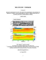
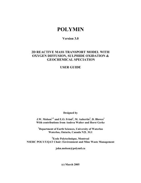
<strong>POLYMIN</strong><br />
Version 3.0<br />
2D REACTIVE MASS TRANSPORT MODEL WITH<br />
OXYGEN DIFFUSION, SULPHIDE OXIDATION &<br />
GEOCHEMICAL SPECIATION<br />
USER GUIDE<br />
Designed by<br />
J.W. Molson 1,2 and E.O. Frind 1 , M. Aubertin 2 , D. Blowes 1<br />
With contributions from Andrea Walter and Horst Gerke<br />
1 Department <strong>of</strong> Earth Sciences, <strong>University</strong> <strong>of</strong> <strong>Waterloo</strong><br />
<strong>Waterloo</strong>, Ontario, Canada N2L 3G1<br />
2 Ecole Polytechnique, Montreal<br />
NSERC POLY/UQAT Chair: Environment and Mine Waste Management<br />
john.molson@polymtl.ca<br />
(c) March 2005
<strong>POLYMIN</strong> 2005<br />
License Agreement<br />
I. Copyright Notice<br />
This s<strong>of</strong>tware is protected by both Canadian copyright law and international treaty<br />
provisions. Therefore, you must treat this s<strong>of</strong>tware just like a book, with the following single<br />
exception. The <strong>University</strong> <strong>of</strong> <strong>Waterloo</strong> (UW) and Ecole Polytechnique (EP) authorize you to make<br />
archive copies <strong>of</strong> the s<strong>of</strong>tware for the sole purpose <strong>of</strong> backing-up our s<strong>of</strong>tware and protecting your<br />
investment from loss.<br />
By saying "just like a book", it is meant for example, that this s<strong>of</strong>tware may be used by any<br />
number <strong>of</strong> people and may be freely moved from one computer location to another, so long as there<br />
is no possibility <strong>of</strong> it being used at one location while it is being used at another. This restriction is<br />
similar to that in publishing where a book for example, can't be read by two different people in two<br />
different places at the same time.<br />
II. Warranty<br />
UW and EP warrant the physical disks and documentation enclosed herein to be free <strong>of</strong><br />
defects in materials and workmanship for a period <strong>of</strong> 30 days from the date <strong>of</strong> purchase. In the event<br />
<strong>of</strong> notification <strong>of</strong> defects in material or workmanship, UW or EP will replace the defective disks or<br />
documentation. The remedy for breach <strong>of</strong> this warranty shall be limited to replacement and shall not<br />
encompass any other damages, including but not limited to loss <strong>of</strong> pr<strong>of</strong>it, and special, incidental,<br />
consequential, or other similar claims.<br />
III. Disclaimer<br />
Neither the developers <strong>of</strong> this s<strong>of</strong>tware, nor any person or organization acting on behalf <strong>of</strong><br />
them makes any warranty, express or implied, with respect to this s<strong>of</strong>tware; or assumes any<br />
liabilities with respect to the use, or misuse, <strong>of</strong> this s<strong>of</strong>tware, or the interpretation, or<br />
misinterpretation, <strong>of</strong> any results obtained from this s<strong>of</strong>tware, or for damages resulting from the use<br />
<strong>of</strong> this s<strong>of</strong>tware.<br />
IV. Governing Law<br />
This license agreement shall be construed, interpreted, and governed by the laws <strong>of</strong> the<br />
Province <strong>of</strong> Ontario, Canada.<br />
2
<strong>POLYMIN</strong> 2005<br />
TABLE OF CONTENTS<br />
page<br />
LIST OF FIGURES....................................................................................................................... 4<br />
LIST OF TABLES ......................................................................................................................... 4<br />
1. INTRODUCTION...................................................................................................................... 5<br />
1.1 Overview............................................................................................................................................5<br />
1.2 Capabilities, Assumptions and Limitations....................................................................................6<br />
1.3 S<strong>of</strong>tware Support..............................................................................................................................7<br />
2. THEORETICAL DEVELOPMENT ......................................................................................... 8<br />
2.1 Background .......................................................................................................................................8<br />
2.2 Mass Transport.................................................................................................................................8<br />
2.3 Primary Variables and their Dimensions .....................................................................................19<br />
2.4 Geochemical Database ...................................................................................................................20<br />
2.5 Input/Output File Definition..........................................................................................................21<br />
3. DESIGNING A MODEL ......................................................................................................... 22<br />
Grid Definition & Boundary Conditions.......................................................................................................22<br />
4. SAMPLE DATA SET............................................................................................................... 25<br />
Input options .................................................................................................................................................27<br />
Grid parameters.............................................................................................................................................28<br />
Data Block 1..................................................................................................................................................29<br />
Print output <strong>of</strong> components ...........................................................................................................................30<br />
Tolerance and relative values........................................................................................................................31<br />
Oxidation Parameters ....................................................................................................................................31<br />
Breakthrough points......................................................................................................................................32<br />
Time Step Data..............................................................................................................................................32<br />
Background aqueous chemistry ....................................................................................................................33<br />
Background solid chemistry..........................................................................................................................34<br />
5. STEP BY STEP INSTRUCTIONS.......................................................................................... 37<br />
6. TIPS AND TECHNIQUES ..................................................................................................... 39<br />
7. PROBLEM DIAGNOSIS AND SOLUTIONS........................................................................ 40<br />
8. REFERENCES ........................................................................................................................ 41<br />
3
<strong>POLYMIN</strong> 2005<br />
LIST OF FIGURES<br />
Figure<br />
page<br />
1. Conceptual domain for <strong>POLYMIN</strong> model applications ................................ 6<br />
2. Simplified <strong>POLYMIN</strong> flowchart .............................................. 16<br />
3. Typical boundary condition configuration. .............................................. 24<br />
4. Typical node and element numbering convention .............................................................. 24<br />
LIST OF TABLES<br />
Table<br />
page<br />
1. Capabilities, assumptions and limitations ................................................... 5<br />
2. Input/Output file definition ........................................................ 21<br />
3. Boundary condition identification ............................................................... 23<br />
4. Problem Diagnosis ...................................................................... 40<br />
4
<strong>POLYMIN</strong> 2005<br />
1. INTRODUCTION<br />
1.1 Overview<br />
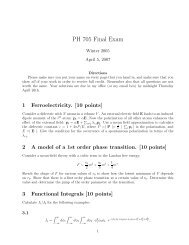
<strong>POLYMIN</strong> is an advanced numerical model for solving reactive mass transport problems. The<br />
model can be used to solve one or two-dimensional mass transport problems within a variety <strong>of</strong><br />
hydrogeological systems. <strong>POLYMIN</strong> was originally developed as a research tool to study the<br />
behaviour <strong>of</strong> acid mine drainage or reactive contaminant plumes within porous media (see Figure 1).<br />
recharge<br />
waste lagoon<br />
monitor well<br />
flow<br />
2000 ppm Cl<br />
shrinking core model<br />
R<br />
r c<br />
C L<br />
recharge<br />
q=0.365m/yr<br />
O 2<br />
Diffusion<br />
sulphurcontining<br />
grain<br />
sand (SBL)<br />
gravel (GRV)<br />
10m<br />
free drainage<br />
Figure 1. Conceptual model domains for the <strong>POLYMIN</strong> model; top: contaminant plume, bottom:<br />
oxidizing rock waste pile (after Molson et al., 2005).<br />
<strong>POLYMIN</strong> will run on any computer although it is recommended that the model be run on at least a<br />
Pentium III/500 MHz machine. The memory requirements depend on your application. 2D<br />
simulations may require on the order <strong>of</strong> 64-128 Mbytes.<br />
5
<strong>POLYMIN</strong> 2005<br />
<strong>POLYMIN</strong> has been developed with some <strong>of</strong> the most efficient and powerful numerical algorithms<br />
available. Finite elements are employed for high accuracy and to allow deformable domain<br />
geometry, and the Leismann time-weighting scheme (Leismann and Frind, 1989) has been<br />
incorporated to maintain matrix symmetry which saves memory and execution time. The model<br />
includes one <strong>of</strong> the most efficient preconditioned conjugate gradient solvers available to solve the<br />
matrix equations.<br />
Custom versions, and executables are available to suit individual needs. Please contact the authors<br />
for available updates. A more recent model, BIONAPL/3D, can also simulate density flow along<br />
with multiple-component NAPL dissolution and reactive transport (Molson, 2001). The <strong>POLYMIN</strong><br />
model has most recently been applied by Molson et al. (2005) to waste rock piles, based on flow<br />
systems developed by Fala et al. (2005).<br />
1.2 Capabilities, Assumptions and Limitations<br />
The capabilities <strong>of</strong> <strong>POLYMIN</strong>, and its major assumptions and limitations are summarized in Table<br />
1.<br />
Table 1. Summary <strong>of</strong> the capabilities, assumptions and limitations <strong>of</strong> <strong>POLYMIN</strong>.<br />
Capabilities<br />
- 2D or 1D domains.<br />
- fully coupled oxygen diffusion, geochemical<br />
speciation and advective-dispersive mass<br />
transport.<br />
- domain can be heterogeneous and<br />
anisotropic.<br />
- deformable elements can conform to<br />
complex geometry.<br />
- versatile boundary condition options.<br />
- computes concentration breakthrough data<br />
(conc. vs time) at selected points.<br />
Assumptions and Limitations<br />
- non-deforming, isothermal aquifer<br />
- fluid is incompressible.<br />
- chemical reactions are assumed at equilibrium<br />
- flow system read separately<br />
- non-fractured or equivalent porous media (2)<br />
(2)<br />
Research versions also available with 1D and 2D fractures (Yang et al, 1996a,b).<br />
6
<strong>POLYMIN</strong> 2005<br />
1.3 S<strong>of</strong>tware Support<br />
If you have questions or comments concerning <strong>POLYMIN</strong>, or this manual, please contact the<br />
authors at the following address:<br />
John Molson / Dr. E.O. Frind<br />
Department <strong>of</strong> Earth Sciences<br />
<strong>University</strong> <strong>of</strong> <strong>Waterloo</strong><br />
<strong>Waterloo</strong>, Ontario, Canada<br />
N2L 3G1<br />
phone: (519) 888-4567 x3959<br />
fax: (519) 746-7484<br />
email: molson@uwaterloo.ca<br />
www: http://sciborg.uwaterloo.ca/~molson/<br />
Montreal address:<br />
J.W. Molson Ph.D. P.Eng.<br />
Dept. <strong>of</strong> Civil, Geological and Mining Engineering<br />
Ecole Polytechnique, Montreal<br />
john.molson@polymtl.ca<br />
http://www.enviro-geremi.polymtl.ca/<br />
Office: (514) 340-4711 x5189<br />
Home: (514) 935-0610<br />
Adjunct Pr<strong>of</strong>essor, <strong>University</strong> <strong>of</strong> <strong>Waterloo</strong><br />
molson@uwaterloo.ca<br />
http://sciborg.uwaterloo.ca/~molson/<br />
John.Molson@polymtl.ca<br />
We would also appreciate hearing about your particular model application and suggestions for<br />
improvement.<br />
7
<strong>POLYMIN</strong> 2005<br />
2. THEORETICAL DEVELOPMENT<br />
2.1 Background<br />
<strong>POLYMIN</strong> is based on the solutions to the 2D advective-dispersive mass transport equation.<br />
The flow field must be generated by a separate program such as FLONET (Molson & Frind,<br />
2004), however other codes can be used as well, provided the grid is compatible. This version <strong>of</strong><br />
the <strong>POLYMIN</strong> model can read the flow system from either the 2D flow model HYDRUS<br />
(Simunek et al., 1999), or from the 2D saturated flow model FLONET (Molson & Frind, 2004).<br />
(see section 4 for a step-by-step list <strong>of</strong> how to run the code)<br />
2.2 Mass Transport<br />
Mass transport is governed by the advection-dispersion equation which includes a source/sink<br />
term for equilibrium reactions. The transport equation in <strong>POLYMIN</strong> for aqueous component k (k<br />
= 1, ..., N c , where N c is the number <strong>of</strong> components) is <strong>of</strong> the form:<br />
∂ θ w C<br />
∂ t<br />
k<br />
∂ ⎛<br />
= ⎜<br />
w D<br />
x<br />
θ<br />
∂ i ⎝<br />
ij<br />
∂ C<br />
∂ x<br />
k<br />
j<br />
⎞<br />
⎟<br />
⎠<br />
-<br />
∂<br />
∂ x<br />
i<br />
( q Ck) + R<br />
i<br />
k<br />
(1)<br />
where C k is the concentration <strong>of</strong> the k th component in the pore water [ML -3 ], q i is the i th<br />
component <strong>of</strong> the volumetric water flux [LT -1 ], D ij is the dispersion coefficient tensor [L 2 T -1 ],<br />
and R k is the source/sink term for the k th component resulting from geochemical equilibrium<br />
reactions [ML -3 T -1 ]. The components <strong>of</strong> the dispersion tensor, D ij , are given by:<br />
θ w Dij<br />
= αT<br />
|q| δ ij + ( α L -α<br />
T<br />
q<br />
j<br />
qi<br />
) + θ Dd<br />
τ δ ij<br />
|q|<br />
(2)<br />
where D d is the molecular diffusion coefficient in water [L 2 T -1 ], ⏐q⏐ is the absolute value <strong>of</strong> the<br />
Darcy fluid flux [LT -1 ], δ ij is the Kronecker delta function, α L is the longitudinal and α T the<br />
transverse dispersivity [L], and τ = θ 7/3 /θ s 2 is a tortuosity factor according to Millington and<br />
Quirk (1961). The tortuosity factor was incorporated into the transport equation to account for<br />
solute diffusion with a spatially variable water content.<br />
Changes to the solid phase due to precipitation-dissolution and sorption-desorption reactions are<br />
represented in <strong>POLYMIN</strong> by the mass conservation equation:<br />
∂ S<br />
∂t<br />
k<br />
= R<br />
S<br />
k<br />
(3)<br />
8
<strong>POLYMIN</strong> 2005<br />
where S k is the solid phase concentration <strong>of</strong> the k th solid component, [ML -3 ], and R k S represents<br />
the change in the k th solid component concentration [ML -3 T -1 ]. Further details are provided by<br />
Walter et al. (1994a).<br />
Oxygen Diffusion<br />
Assuming an immobile air phase (convection is neglected), oxygen transport through the<br />
unsaturated porous medium is governed by the 2D equation for oxygen diffusion, expressed as:<br />
θ<br />
eq<br />
2 2<br />
∂ [ O2 ]<br />
a<br />
⎛ ∂ [ O2 ]<br />
a ∂ [ O2<br />
]<br />
a<br />
⎞<br />
= D e ⎜ + - Q<br />
2 2 ⎟<br />
∂t ⎝ ∂ x ∂ z ⎠<br />
O 2<br />
(4)<br />
where θ eq (x,z,t) is the spatially and temporally-variable water phase corrected volumetric air<br />
content [-], D e (x,z,t) is the effective oxygen diffusion coefficient [L 2 T -1 ], and Q O2 (x,z,t) is the<br />
sink term for oxygen consumption due to sulphide mineral oxidation (M O2 /L 3 /T) (see below).<br />
The equivalent air content θ eq in Equation (4) is defined here as θ eq = θ a + Hθ w where θ a is the<br />
air-filled porosity and H is Henry’s Law coefficient for equilibrium oxygen partitioning between<br />
air and water (-). The oxygen diffusion coefficient D e is represented in <strong>POLYMIN</strong> by the Aachib<br />
et al. (2002) model:<br />
D<br />
e<br />
1 ⎡ p D<br />
a w pw<br />
= ⎢Daθ<br />
a<br />
+ θ<br />
w<br />
θ 2<br />
⎣ H<br />
s<br />
⎤<br />
⎥<br />
⎦<br />
(5)<br />
where D a and D w are the diffusion coefficients in air and water, respectively, and p a and p w are<br />
fitting coefficients; here p a = p w = 3.3 is assumed, as suggested by Aachib et al. (2002).<br />
The coefficient D e , representing diffusion within the air-filled porosity <strong>of</strong> the unsaturated spoil,<br />
can be represented using models presented by Elberling & Nicholson (1993), Millington &<br />
Quirk (1961), or Aachib et al. (2002).<br />
Sulphide Oxidation<br />
Acid mine drainage is controlled by the oxidation <strong>of</strong> sulphide minerals, mostly pyrite and<br />
pyrrhotite, within the waste rock. The oxidation <strong>of</strong> pyrite, for example, can be described in<br />
simplified form by the following stoichiometric equations (Wunderly et al, 1996):<br />
2+<br />
2- +<br />
Fe S 2 + H 2 O +7/2 O2<br />
⇒ Fe + 2 SO4<br />
+ 2 H<br />
9
<strong>POLYMIN</strong> 2005<br />
2+<br />
+ 3+<br />
Fe +1/4 O2<br />
+ H ⇒ Fe +1/2 H 2 O<br />
3+ 2- +<br />
Fe S 2 +1/2 H 2 O +15/4 O2<br />
⇒ Fe + 2 SO4<br />
+ H<br />
The rate <strong>of</strong> these oxidation reactions, however, is controlled by the availability <strong>of</strong> oxygen at, and<br />
within the mineral grains. A common approach for modeling this process, and that adopted here,<br />
is the shrinking core model (Levenspiel, 1972) which assumes the sulphide mineral is<br />
uniformally distributed within each spherical grain. Derivations for this model have been<br />
presented by Davis and Ritchie (1986; 1987), Wunderly et al. (1996), and Gerke et al. (1998),<br />
and are not repeated here.<br />
The shrinking core model provides the oxygen sink term Q o in equation (4), defined by<br />
3 ( 1 - θ ) ⎛ r ⎞ [ O 2 ]<br />
R ⎝ r ⎠ H<br />
c<br />
o<br />
= 2 2 ⎜<br />
R -<br />
⎟<br />
c<br />
Q D<br />
a<br />
(6)<br />
where D 2 is the effective diffusion coefficient incorporating the characteristic diffusion<br />
properties <strong>of</strong> both the water film and the oxidized shell <strong>of</strong> the pyrite particle, R is the average<br />
radius <strong>of</strong> the soil particles, r c is the average radius <strong>of</strong> the unreacted core, and [O 2 ] a is the oxygen<br />
concentration in the air phase in contact with the particle.<br />
From the computed change in the oxidized grain radius (r c ), and knowing the fraction <strong>of</strong> sulfide<br />
minerals in the grain f s , (M Su /M solids ), the bulk density ρ b [ML -3 ], and ε, the mass ratio <strong>of</strong> oxygen<br />
to sulphur consumed on the basis <strong>of</strong> the reaction stoichiometry, the mass <strong>of</strong> each oxidation<br />
product can be determined for each oxidation time step ∆t oxid (Gerke et al., 1998).<br />
Geochemical Equilibrium Equations<br />
The chemical equilibrium reactions are those provided in the geochemical equilibrium model<br />
MINTEQA2 (Felmy et al., 1983; Allison et al., 1990). MINTEQA2 was derived from combining<br />
the geochemical equilibrium model MINEQL (Westall et al., 1976) with the data base <strong>of</strong> the<br />
WATEQ2 model (Ball et al., 1979).<br />
The reactions considered are chemical speciation, acid-base reactions, mineral precipitationdissolution,<br />
oxidation-reduction, and adsorption. The chemical model uses the general<br />
transformation-<strong>of</strong>-the-bases mathematical approach to solve the chemical equilibrium problem<br />
for all <strong>of</strong> the chemical reaction types (Felmy et al., 1983). The ion-association equilibriumconstant<br />
approach is used to represent the geochemical reactions. The ion-association aqueous<br />
10
<strong>POLYMIN</strong> 2005<br />
model involves three separate constituents; the masses <strong>of</strong> aqueous species and complexes,<br />
equilibrium constants which relate these complexes in solution, and the individual ion-activity<br />
coefficients for each species. These constituents are related through a system <strong>of</strong> algebraic<br />
equations that solve for the individual ion activities in a solution, which are in turn used to<br />
predict chemical reaction equilibrium.<br />
Chemical Speciation, Acid-Base Reactions and Redox Reactions<br />
In a solution, there exists a set <strong>of</strong> chemical components and species. The set <strong>of</strong> chemical<br />
components is the minimum number <strong>of</strong> species that uniquely describe a solution and that is<br />
required to be reaction invariant (Mangold and Tsang, 1991). The component mass remains<br />
constant, regardless <strong>of</strong> the distribution between chemical species in both the aqueous and solid<br />
phases. This mass conservation principle yields a set <strong>of</strong> linear algebraic equations, with one<br />
equation for each component (Cederberg, 1985).<br />
The total component concentration T k (moles/1000g H 2 O) is the sum <strong>of</strong> the aqueous-phase<br />
concentration C k and the solid-phase concentration S k , <strong>of</strong> component k:<br />
T k = Ck<br />
+ S k<br />
(7)<br />
where<br />
C<br />
S<br />
k<br />
k<br />
naq<br />
alk<br />
∑ cl<br />
(8)<br />
l=1<br />
= k = 1, ... N<br />
=<br />
naq<br />
blk<br />
∑ s<br />
k = 1,...<br />
l<br />
N<br />
(9)<br />
l=1<br />
and where c l is the concentration <strong>of</strong> species l in the aqueous phase (moles/1000g H 2 0), s l is the<br />
concentration <strong>of</strong> species l in the solid phase (moles/1000g H 2 O), a lk is the stoichiometric<br />
coefficient <strong>of</strong> component k in species c l , b lk is the stoichiometric coefficient <strong>of</strong> component k in<br />
species s l , n aq is the number <strong>of</strong> species in the aqueous phase, and n s is the number <strong>of</strong> species in<br />
the solid phase.<br />
The total mass <strong>of</strong> each chemical component must be known to describe a solution. The<br />
distribution <strong>of</strong> the species included in the component concentrations is estimated by mass-action<br />
equations that form a set <strong>of</strong> nonlinear algebraic equations, with one equation for each chemical<br />
species. For the aqueous-phase species, these equations are:<br />
N c<br />
alk<br />
χ = K ∏ χ<br />
naq<br />
(10)<br />
l<br />
cl<br />
k=1<br />
k<br />
while for the solid-phase species, they are:<br />
l = 1,...<br />
11
<strong>POLYMIN</strong> 2005<br />
sl<br />
= K<br />
N<br />
c<br />
blk<br />
∏ χ k<br />
ns<br />
(11)<br />
sl<br />
k=1<br />
l = 1,...<br />
where K cl is the equilibrium formation constant for species c l , K sl is the equilibrium formation<br />
constant for species s l in the solid phase, χ k is the activity <strong>of</strong> component k (moles/1000g H 2 0),<br />
and χ l is the activity <strong>of</strong> species l (moles/1000g H 2 0).<br />
The stoichiometric mass-balance equations for the components are written in terms <strong>of</strong><br />
component concentrations, while the mass action equations are expressed in terms <strong>of</strong> activities.<br />
The activities, χ l , are related to concentrations, c l , through the individual ionic activity<br />
coefficients, γ l , using the approximation<br />
χ = cl<br />
(12)<br />
l<br />
γ l<br />
The activity coefficients are calculated using the WATEQ, extended Debye-Hückel or Davies<br />
equations (Felmy et al. 1983). The specific equation used is dependent on the availability <strong>of</strong><br />
specific solute parameters.<br />
These equations form a set <strong>of</strong> algebraic equations which are used in the ion-association model to<br />
solve for the individual ion activities given the total component concentrations in solution. The<br />
interrelationships between the species concentrations and activities and the ionic strength cannot<br />
be solved for explicitly but require an iterative solution. MINTEQ uses the Newton-Raphson<br />
iterative technique.<br />
Chemical reactions involving the hydrogen and hydroxide ion are simulated in the chemical<br />
model using the proton condition (Westall et al., 1976; Felmy et al., 1983; Allison et al., 1990).<br />
The proton condition, representing the total analytical component concentration <strong>of</strong> H + , is the<br />
primary variable used in the transport solution. The H + -value may theoretically be negative<br />
because it does not have the physical interpretation <strong>of</strong> a total mass <strong>of</strong> hydrogen but is the change<br />
in H + activity from the reference condition. Similarly, the total calculated mass <strong>of</strong> H 2 O can also<br />
be negative.<br />
Oxidation-reduction reactions are calculated with MINTEQ using the external redox couple<br />
approach. This approach requires that the initial distribution <strong>of</strong> the specified redox couples is<br />
known before the chemical equilibrium problem can be solved. This distribution can be<br />
determined from the initial solution component chemistry and the solution pe. MINTEQ permits<br />
selection <strong>of</strong> redox couples that are set in equilibrium with the solution pe. Other electroactive<br />
species may be considered independent <strong>of</strong> the pe. Thus, the multivalent species can be reacted<br />
with their respective solid mineral phases without requiring interactions with other multivalent<br />
species. In the present transport model, the total dissolved concentration <strong>of</strong> each redox state is<br />
transported separately, and the new solution pe is calculated using the activities calculated for<br />
the specified redox couples at the new location. The electron activity, therefore, is not transported<br />
independently.<br />
Sorption<br />
12
<strong>POLYMIN</strong> 2005<br />
The three basic mathematical forms <strong>of</strong> sorption reaction models, namely isothermal, massaction/ion-exchange,<br />
and surface complexation/electrostatic models, have been incorporated into<br />
MINTEQ (Allison et al., 1990). The isothermal models included are the activity K d adsorption<br />
model, the activity Langmuir adsorption model, and the Freundlich model. The electrostatic<br />
adsorption models available are the constant-capacitance model, the diffuse-layer model, and the<br />
triple-layer model. To date only the ion-exchange model has been verified in the combined<br />
mass-transport chemical-equilibrium model.<br />
Ion-exchange sorption reactions are simulated using the Gaines and Thomas model for ion<br />
exchange (Allison et al., 1990). This model assumes that the surface site is initially occupied by<br />
an exchangeable ion that is released into solution during the exchange process, that the charge on<br />
the surface <strong>of</strong> the solid remains constant, and that the number <strong>of</strong> surface sites available for<br />
sorption, expressed as the cation exchange capacity (C.E.C.), is fixed. The ion-exchange<br />
reaction is written as:<br />
vA<br />
vB<br />
B + AB(ad) ⇔ B A(ad) + A<br />
(13)<br />
v A v v v<br />
B<br />
where v A and v B are the change on components A and B respectively, A(ad) and B(ad) are the<br />
adsorbed mass <strong>of</strong> components A and B. The mass action equation for the above expression is<br />
K<br />
AB<br />
⎛ A(ad)<br />
= ⎜<br />
vA<br />
⎝ [A ]<br />
⎞<br />
⎟<br />
⎠<br />
vB<br />
vB<br />
⎛ [B ]<br />
⎜<br />
⎝ B(ad)<br />
⎞<br />
⎟<br />
⎠<br />
vA<br />
(14)<br />
where the square brackets represent solution activity, and K AB is the selectivity coefficient <strong>of</strong><br />
species A with respect to species B.<br />
Mineral Precipitation and Dissolution<br />
Mass-action equations, which relate ion activities and a solid specific solubility product, describe<br />
mineral precipitation and dissolution reactions. These reactions can be written as follows (Walter<br />
et al., 1994a):<br />
A a<br />
B b(s)<br />
⇔ aA (aq)<br />
+ bB (aq)<br />
(15)<br />
The subscripts (s) and (aq) refer to solid and aqueous phases respectively. The thermodynamic<br />
solubility product for a given solid is described by:<br />
K<br />
sp<br />
a<br />
A B<br />
= [ ] [ ]<br />
[ AB]<br />
a<br />
b<br />
b<br />
(16)<br />
where K sp<br />
is the solubility product for the solid.<br />
13
<strong>POLYMIN</strong> 2005<br />
⎛ I.A.P. ⎞<br />
S.I.= log ⎜ ⎟<br />
(17)<br />
⎝ K sp ⎠<br />
If the saturation index is greater than zero, representing supersaturation, there is a tendency for<br />
the mineral to precipitate. When the S.I. is zero, the mineral and the solution are in equilibrium.<br />
If the S.I. is less than zero the mineral is undersaturated, and the tendency is for the mineral to<br />
dissolve. In real geochemical situations, minerals which are super-saturated or undersaturated<br />
may not precipitate or dissolve due to kinetic limitations. These limitations are not addressed in<br />
the current model.<br />
The solid phases incorporated in the data base may be designated as one <strong>of</strong> three types:<br />
1. A solid which is in infinite supply (reacted to equilibrium),<br />
2. A solid with a finite supply where the initial amount <strong>of</strong> solid must be specified (moles <strong>of</strong><br />
solid per litre <strong>of</strong> pore water), and<br />
3. A dissolved solid which may precipitate if it becomes supersaturated.<br />
Within an individual chemical simulation, the designation may switch between the last two solid<br />
types. This occurs when a finite-mass solid is completely dissolved, becoming a dissolved solid.<br />
The solid type change is accounted for in the combined chemical-transport model to allow<br />
complete mineral dissolution at an individual node within the spatial domain at any point in time.<br />
Switching solid types is well suited to the coupled geochemical-reaction, solute-transport<br />
problems where sharp changes in solid-phase concentrations may be observed.<br />
The determination <strong>of</strong> solids that are thermodynamically stable from the array <strong>of</strong> solids allowed to<br />
precipitate or dissolve is calculated by treating the S.I. (eq. 14) as an inequality. Each solid is<br />
ranked for its tendency to precipitate by dividing the S.I. by the number <strong>of</strong> ions in the solid<br />
formation reaction. After ranking, the solid with the highest value is allowed to precipitate. All<br />
<strong>of</strong> the remaining solids are then ranked again and sequentially precipitated or dissolved until all<br />
<strong>of</strong> the solids considered are undersaturated. A provision is made to insure that if the mass <strong>of</strong> the<br />
previously precipitated solid becomes negative, that solid will redissolve and the solution<br />
procedure will continue.<br />
Limitations <strong>of</strong> Geochemical Model<br />
The ion-association model used in MINTEQ to account from deviations from chemical ideality<br />
is valid only for low ionic strengths <strong>of</strong> 0 - 0.5. The previously-described chemical reactions are<br />
all based on the L.E.A. This assumption means that the reactions modelled are sufficiently rapid<br />
relative to the contaminant travel times through the reacting medium, or that a reaction will go to<br />
equilibrium before a component is transported to another point in space. On a purely<br />
geochemical basis, the majority <strong>of</strong> the reactions considered in this study adhere to the L.E.A.,<br />
with the possible exception <strong>of</strong> some solid and redox reactions which are <strong>of</strong>ten rate-dependent.<br />
The field results presented by Morin (1983) suggest that both the use <strong>of</strong> the ion-association<br />
model and the L.E.A. are reasonable at the Nordic Site.<br />
14
<strong>POLYMIN</strong> 2005<br />
Solution Strategy<br />
<strong>POLYMIN</strong> uses two-step sequential physical-chemical coupling (Walter et al, 1994a) to solve<br />
the reactive transport equations. In this approach, the transport equation is split into a physical<br />
step, and a chemical step:<br />
Step 1 (physical)<br />
n+1 phys<br />
equil<br />
( C k - Ck<br />
) δ(t + ∆t)= Rk<br />
δ(t + ∆t)<br />
k = 1,...,N c<br />
(18)<br />
Step 2 (chemical)<br />
( C<br />
- C<br />
∆t<br />
phys<br />
k<br />
n<br />
k<br />
)<br />
= L( C<br />
k<br />
)<br />
n+1/2<br />
k = 1,...,N<br />
c<br />
(19)<br />
where C k phys is the concentration <strong>of</strong> component k at the end <strong>of</strong> the physical step, L represents the<br />
transport operator, δ is the Dirac delta, and n, n+1/2, n+1 relate to the beginning, midpoint, and<br />
end <strong>of</strong> the time step ∆t, respectively.<br />
The transport model is coupled to the oxygen diffusion and pyrite oxidation modules following<br />
the sequence shown in Figure 1. The simulation over a transport time step ∆t begins with an<br />
iterative solution to the oxygen diffusion and reactive core equations which liberates H + , SO 4 2+ ,<br />
Fe 2+ and Fe 3+ . Because <strong>of</strong> the nonlinearity for these coupled reactions, the solution is performed<br />
over a smaller sub-time step ∆t oxid , typically 1/10 th - 1/50 th <strong>of</strong> the transport time step ∆t. These<br />
calculations are very rapid and do not significantly affect the total execution time. The reactive<br />
products are accumulated over each sub-time interval and are added to the existing nodal<br />
concentrations just before the chemical equilibration step.<br />
Following convergence <strong>of</strong> the diffusion and reactive core equations, a second iterative sequence<br />
begins for the physical/chemical steps. The accumulated oxidation products are added to C k<br />
phys<br />
following the transport step. The equilibrium chemical step is completed independently for each<br />
grid node. An option is available for automatically bypassing this step if the changes in<br />
concentration from the transport and oxidation steps are below a threshold. Typically, the<br />
transport and chemical steps account for approximately 1/3 rd and 2/3 rd <strong>of</strong> the total execution<br />
time, respectively. Execution times for a 50-year, 13,657-node simulation using a Pentium IV,<br />
3.3Ghz machine were on the order <strong>of</strong> 40 hours.<br />
15
<strong>POLYMIN</strong> 2005<br />
Transport/Reaction time step ∆t<br />
Oxidation time step (∆t oxid =∆t/20)<br />
Solve oxygen diffusion (O 2<br />
)<br />
Solve core oxidation (r c<br />
)<br />
[O 2<br />
] Converged?<br />
no<br />
yes<br />
Accumulate reaction products (SO 4 2+ , Fe 2+ , Fe 3+ , H + )<br />
Solve physical transport step<br />
Solve chemical step<br />
Components Converged?<br />
no<br />
yes<br />
Figure 2. Flowchart <strong>of</strong> the Polymin model.<br />
16
<strong>POLYMIN</strong> 2005<br />
Discretization Criteria<br />
Accuracy and stability criteria for the numerical solution <strong>of</strong> multi-component reactive<br />
transport problems are not yet well defined. The basic requirements, which apply to linear<br />
transport <strong>of</strong> nonreactive solutes with linear retardation are the Peclet and Courant criteria (Daus<br />
et al., 1985):<br />
Pe=<br />
Co=<br />
v ∆L<br />
≤ 2<br />
D<br />
v ∆t<br />
≤<br />
∆x<br />
Pe<br />
2<br />
(20)<br />
(21)<br />
where v and D are the velocity and dispersion coefficient in the principal (flow) direction,<br />
respectively, ∆L is the effective element length in the flow direction, and ∆t is the time step. In<br />
order to control numerical dispersion and oscillations, eq. (18) is used to constrain the spatial<br />
discretization, while eq. (19) is used to constrain the time step.<br />
In nonreactive transport applications, the Peclet and Courant constraints are <strong>of</strong>ten exceeded by a<br />
factor <strong>of</strong> 2 to 4 since the resulting small oscillations are generally harmless. In reactive<br />
transport, on the other hand, numerical oscillations are more problematic since negative concentrations<br />
can be fatal for the chemical equilibrium model. Some authors eliminate oscillations at<br />
the cost <strong>of</strong> smearing by using upwinding; we do not recommend this procedure because the<br />
smearing causes fictitious reactions ahead <strong>of</strong> the actual concentration front. Instead, we seek to<br />
maintain second-order accuracy (or equivalent) in time through time-centred weighting throughout.<br />
Numerical oscillations are controlled by satisfying criteria (19) and (20) everywhere.<br />
For reactive transport, constraints arise out <strong>of</strong> the basic requirement that the mass reacted per<br />
time step should be in some reasonable relationship to the mass present. In the case <strong>of</strong> decay or<br />
biodegradation, this requirement leads to a relationship between the time step and the decay<br />
coefficient (Luckner and Schestakov, 1991). For general reactive transport, a useful quantity is<br />
the elemental Damköhler number, defined by Zysset and Stauffer (1992) as the ratio <strong>of</strong> the<br />
advective time t a = ∆L/v to the reactive time t r = C k B /S k , with C k B being some representative<br />
concentration such as the boundary input or the background concentration <strong>of</strong> k, and S k being the<br />
reaction rate.<br />
In the case <strong>of</strong> equilibrium reactions, the reaction rate has no theoretical meaning. We therefore<br />
define the reactive time as:<br />
t<br />
r<br />
=<br />
t+ ∆t<br />
∫<br />
t<br />
t+ ∆t<br />
R<br />
∫ C k dt<br />
t<br />
=<br />
k δ(t+<br />
∆t)<br />
C<br />
k<br />
R<br />
∆t<br />
k<br />
(22)<br />
where C k represents the elemental average concentration over the time step. The Damköhler<br />
17
<strong>POLYMIN</strong> 2005<br />
number is then defined as:<br />
ta<br />
Dak<br />
=<br />
tr<br />
∆L<br />
Rk<br />
=<br />
v C k<br />
∆t<br />
(23)<br />
The product <strong>of</strong> the Courant number and the Damköhler number is used by Zysset and<br />
Stauffer (1992) to express the relationship between the reaction rate and the characteristic<br />
concentration <strong>of</strong> a component. In the case <strong>of</strong> equilibrium reactions, the equivalent quantity is the<br />
reactive mass ratio ρ k , which can be defined relative to the characteristic (background or input)<br />
concentration C k B , as:<br />
B<br />
B<br />
= Co =<br />
Rk<br />
ρ<br />
k<br />
• Dak<br />
(24)<br />
B<br />
C k<br />
Alternatively, the reactive mass ratio can be defined relative to the actual point concentration<br />
at the end <strong>of</strong> the physical step C k phys , as:<br />
C<br />
=<br />
Rk<br />
ρ<br />
k<br />
= Co • Dak<br />
(25)<br />
phys<br />
Ck<br />
Since the reactive mass depends on the time step ∆t, either <strong>of</strong> these relationships can be<br />
used to define a time step constraint. The value <strong>of</strong> such a constraint will depend on the nature <strong>of</strong><br />
the chemical reactions as well as the characteristics <strong>of</strong> the particular chemical reaction routine<br />
used. For fast reversible reactions, Zysset and Stauffer (1992) recommend ρ k B ≤ 0.01. The<br />
MINTEQ-based model generally reached much higher values (see applications below), for the<br />
scenarios investigated.<br />
The reactive mass ratio ρ k C defined by eq. (23) represents the mass generated or consumed<br />
relative to the mass present at the end <strong>of</strong> the physical step. Since the mass consumed (R k ≤ 0)<br />
cannot exceed the mass present, ρ k C ≥ - 1. Upper limits on ρ k B and ρ k C have not yet been defined;<br />
it is to be expected that any such limits will depend on the ability <strong>of</strong> the geochemical model to<br />
equilibrate a perturbed system. By monitoring the performance <strong>of</strong> the model for various<br />
scenarios under different chemical environments, we expect eventually to be able to define<br />
appropriate constraints.<br />
18
<strong>POLYMIN</strong> 2005<br />
2.3 Primary Variables and their Dimensions<br />
The following variables must be dimensioned large enough to accommodate the chosen grid size.<br />
These values are set in the PARAMETER statement within the main program.<br />
Array dimension limits: (see parm.inc, parmt.inc, mintran.inc, minteq.inc)<br />
maxne ....<br />
maxnn ....<br />
maxn ....<br />
maxna ....<br />
laa ....<br />
Nxdim …<br />
Nydim …<br />
Nrdim …<br />
maxbt ....<br />
maxtim ....<br />
maxpt …<br />
Maximum number <strong>of</strong> elements in the transport grid.<br />
Maximum number <strong>of</strong> nodes in the transport grid.<br />
Maximum number <strong>of</strong> degrees <strong>of</strong> freedom (= maxnn - # <strong>of</strong> fixed nodes).<br />
Total number <strong>of</strong> non-zero matrix entries in condensed matrix.<br />
(As a conservative approximation, use maxna = 14 * maxn).<br />
PCG solver matrix dimension.<br />
(As a conservative approximation, use laa = 3*maxn+maxna).<br />
maximum number <strong>of</strong> components<br />
maximum number <strong>of</strong> aqueous species<br />
maximum number <strong>of</strong> solid species<br />
Maximum number <strong>of</strong> "wells" at which breakthrough curves are generated<br />
Maximum number <strong>of</strong> time steps<br />
maximum number <strong>of</strong> print times<br />
Note these values all represent maximum limits, they can be equal to, or greater than, the actual<br />
number required.<br />
A conservative estimate for maxna is 14 x maxn, and since this parameter reserves memory for one<br />
<strong>of</strong> the largest real arrays, it should be minimized if available computer RAM is limited. <strong>POLYMIN</strong><br />
computes the minimum vector length (maxna) required by the flow and transport problems and<br />
writes this information to the listing file (look for "vector length"). For more efficient memory use,<br />
these values can be substituted into the PARAMETER statement. To do this, the model must first be<br />
run using an initial estimate for maxna (and hence laa), at least until the correct vector lengths are<br />
computed. The minimum vector length and new value for laa is then entered into the program,<br />
which is then recompiled and rerun for the full simulation. The code will detect if the given array<br />
limits are too small, in which case the execution will terminate with an error message.<br />
19
<strong>POLYMIN</strong> 2005<br />
Other important variables:<br />
nn<br />
ne<br />
x,y,z<br />
vx,vy,vz<br />
u0,u1,u2<br />
in<br />
........... total number <strong>of</strong> nodes in the finite element grid<br />
........... total number <strong>of</strong> elements in finite element grid<br />
........... nodal grid coordinates<br />
........... elemental average linear groundwater flow velocities<br />
........... nodal concentration arrays (at last time step, most recent iteration, and new<br />
solution respectively)<br />
........... element incidence array<br />
2.4 Geochemical Database<br />
The database files used by <strong>POLYMIN</strong> and their analogous MINTEQA2 files are:<br />
<strong>POLYMIN</strong><br />
alk.dbm<br />
analy.dbm<br />
error.dbm<br />
compcp.dbm<br />
type6cp.dbm<br />
thermcp.dbm<br />
MINTEQA2<br />
alk.dbs<br />
analyt.dbs<br />
error.dbs<br />
comp.dbs<br />
type6.dbs<br />
thermo.dbs<br />
Redox and gas reactions can be included in type6cp.dbm and thermcp.dbm database files<br />
within MINTOX and thus do not have their own database files. Modifications to these database<br />
files can be made relatively easily. They are in ascii format and the format/unformat routine<br />
necessary when modifying MINTEQA2 database files is not needed.<br />
To add a component to the databases edit the compcp.dbm file and insert the new<br />
component in the same format as in the comp.dbs MINTEQA2 file. To add reactions, add the<br />
reaction to both the type6cp.dbm and the thermcp.dbm files in the same format as the reaction<br />
occurs in the MINTEQA2 database files. The <strong>POLYMIN</strong> program does not need to be<br />
recompiled when changes are made to the database files.<br />
20
<strong>POLYMIN</strong> 2005<br />
2.5 Input/Output File Definition<br />
Table 2. Input/Output files used in <strong>POLYMIN</strong>.<br />
Unit # Filename: I/O Contents:<br />
5 polymin.dat I primary input data<br />
5 Polymin.in I name <strong>of</strong> input data file<br />
16 Polymin0.gen O Echoes the input data, prints info while running<br />
various Polymino.aq_ O 2D concentration data for all aqueous components<br />
various Polymino.so_ O 2D concentration data for all solid components<br />
various Brkaq_.out O Breakthrough data (time, concentration) - aqueous<br />
various Brks_.out O Breakthrough data (time, concentration) - aqueous<br />
88 Debug.out O Debug information<br />
2 Thermcp.dbm I Thermodynamic database<br />
3 Compcp.dbm I database<br />
4 Type6cp.dbm I database<br />
10 Alk.dbm I database<br />
7 Analy.dbm I database<br />
13 Error.dbm I database<br />
99 Bckgrndpoly,min I Background concentration data<br />
100 Meshtria.txt I Finite element triangular mesh coordinates, incidences<br />
110 th.txt I Water content<br />
120 Bdy.txt I Boundary nodes<br />
99 Nodeprop.txt I Initial nodal properties (grain radius, porosity, sulphur fraction)<br />
99 v.txt I Element velocities<br />
50 Polymin.ur1 O 2D plotting file for Tecplot (x,z,c k ) – aqueous components<br />
51 Polymin.ur2 O 2D plotting file for Tecplot (x,z,c k ) – solid components<br />
21
<strong>POLYMIN</strong> 2005<br />
3. DESIGNING A MODEL<br />
Grid Definition & Boundary Conditions<br />
<strong>POLYMIN</strong> currently supports a 1D or 2D domain discretized using triangular elements. With<br />
triangular elements, the grid can be unstructured, the connectivity (incidence) information is<br />
provided in the meshtria.txt file.<br />
The grid is generated either with the Flonet (Fnpcg) model, or by Hydrus. In either case, the grid is<br />
imported into <strong>POLYMIN</strong> using the meshtria.txt file.<br />
The element incidence array, which defines the global node numbers connected to each element, is<br />
stored in the array in(l,i) where l is the global element number, and i (=1,2,3) is the local element<br />
node number.<br />
Two examples are provided here to clarify the grid generation procedure. Note these examples are<br />
for demonstration purposes only, and would not be <strong>of</strong> sufficient resolution for a practical application<br />
since the Peclet and Courant criteria would be violated under most situations.<br />
Transport boundary conditions can be 1 st , 2 nd or 3 rd type (Table 3, Fig. 3.). The default is 2 nd type,<br />
zero-gradient. The bdy.txt file is divided into 2 sections: top and bottom boundary nodes. Currently,<br />
the model is restricted to a fixed oxygen concentration across the top, and a zero-gradient oxygen<br />
boundary at the bottom (the O2 conc. Can also be fixed to zero across the bottom boundary nodes<br />
using lo2fix=.true.. For the aqueous components, the top boundary nodes can be either first or thirdtype,<br />
depending on the value <strong>of</strong> kcauchy.<br />
The grid numbering is shown in Fig. 4 (for the case <strong>of</strong> a rectangular grid subdivided into triangles, as<br />
created by FLONET).<br />
22
<strong>POLYMIN</strong> 2005<br />
Table 3.<br />
Summary <strong>of</strong> transport boundary conditions available in <strong>POLYMIN</strong>.<br />
Boundary<br />
Type<br />
Definition<br />
First / Dirichlet c = c 0<br />
Fixed concentration boundary (e.g. a large, wellmixed<br />
source)<br />
Second /<br />
Neumann<br />
∂c = 0<br />
∂n<br />
Zero-concentration gradient (e.g. outflow or<br />
impermeable boundary).<br />
Third / Cauchy q0<br />
0 ∂c<br />
= vc - D<br />
θc<br />
∂ x i<br />
Dispersive flux boundary<br />
(e.g. source with known influx q 0 and<br />
concentration c 0 ).<br />
23
<strong>POLYMIN</strong> 2005<br />
C=1 0<br />
C=0<br />
or<br />
dc/dx=0<br />
C=0 0<br />
dc/dx=0<br />
Dc/dz=0<br />
Z<br />
X<br />
Figure 3. Typical boundary condition configuration.<br />
4<br />
8<br />
12<br />
3<br />
2<br />
1<br />
18<br />
17<br />
2<br />
1<br />
3<br />
4<br />
16<br />
1<br />
1<br />
Element number<br />
Node number<br />
Figure 4. Typical node and element numbering convention for rectangular-based triangle grid.<br />
24
<strong>POLYMIN</strong> 2005<br />
4. SAMPLE DATA SET<br />
The example below is used to illustrate the format <strong>of</strong> the input files polymin.dat and<br />
bckgrndpoly.min. The example is a source <strong>of</strong> low pH water at the watertable <strong>of</strong> an unconfined<br />
aquifer.<br />
We begin with the data file for the FLONET model, which is explained further in the FLONET<br />
manual. The polymin.dat file is explained line-by-line below.<br />
FLONET model datafile:<br />
(refer to Molson & Frind (2004) for the FLONET User Guide.<br />
FLONET: HEAD / STREAM FUNCTION MODEL:<br />
FLOW.DATA - SAMPLE DATA FILE -<br />
November, 2000<br />
0 0 -999. ;SSINK<br />
1 1 0 0 1 0 ;kp,kv,kg,kread,ksolv,khk<br />
101 21 200. 10. 1 1 ;NX,NY,XL,YL,NGX,NGY<br />
0 20 0.01 0. ;maxit,nwtl,tol,datum<br />
0 ;WATERTABLE CODE(KW)<br />
1. 0.0 .00 0.0 -0.05 ;watertable shape<br />
1 1 999 1 10.7 ;BOUNDARY CONDITIONS - left side<br />
2 1 999 0 1.000e-8 ;boundary conditions - top<br />
3 1 999 1 10.0 ;boundary conditions - right side<br />
4 1 999 0 0. ;boundary conditions - bottom<br />
-1 ;END BOUNDARY CONDITIONS<br />
-1 ;END INTERNAL DIR NODES<br />
1 4000 0.5e-4 0.5e-4 0.0 0.35 -1 ;hydraulic K triangle elements!<br />
100. 150. 2. 5. 1.e-3 1.e-3 0. .35 -1 ;high-K lense<br />
0 0 0 0 0.e-4 0.e-4 0. 0.35 -1 ;indexed<br />
25
<strong>POLYMIN</strong> 2005<br />
Sample <strong>POLYMIN</strong> Input Data File (polymin.dat)<br />
Poly triangle version<br />
1.0 0.5 0.0 ;WP,WA,WB,Leissman terms<br />
0 50.0 0 0 1 0 0 ;KMAS,PTIME,KTS,kiter,kbypass,kint,kdim=1 axisymmetric<br />
0 7 2 0 0 ;KPRT,NPRT,LPRT,N1,N2<br />
0.1 0.5 1. 5. 10. 20. 50. ;(PRNTT(I),I=1,NPRT)<br />
200 20 2 9 ;NEX,NEZ,NVTYP,NGTYP<br />
40. 50. 1000. ;XL,ZL,CONF<br />
0.06 0.35 10. 1836. .0003 0.9 ;core: fs2i,por2i,temp2i,rhob2i,ox1i,uradius1i<br />
0 0 0 ;IS1,IS2,NCHS<br />
0. 0. false ;vx,vz,ln<strong>of</strong>lx(t: zero water velocity)<br />
0.5 0.05 0.005046 ;Al,At,DD<br />
10.0 0.0 14 8 0 ;TEMP,FIONS,NNN,NR,NAS<br />
0 0 3 0 4 0 0 0 0 0 0 ;IFL(11)<br />
0 0 0 ;IADS,NUMADS,IABG<br />
0 ;ntsn<br />
1 1 2 2 3 3 4 4 5 5 6 6 7 0 0 0 ;KPLT(I),I=1,NNN<br />
0 1 2 3 4 5 6 7 0 0 0 0 ;KPLTS(I),I=1,NR<br />
1 1 1 1 1 1 1 1 1 1 1 1 1 1 1 0 ;KPNT(I),I=1,NNN<br />
1 1 1 1 1 1 1 1 1 1 1 0 ;KPNTS(I),I=1,NR<br />
2.000E-03 1.375E-02 ;CA TOLERANCE AND RELATIVE VALUES<br />
2.000E-03 2.490E-02 ;MG FROM NICKEL3<br />
2.000E-03 1.093E-02 ;NA "<br />
2.000E-03 5.140E-03 ;K "<br />
2.000E-03 4.252E-04 ;CL "<br />
2.000E-03 1.380E-02 ;CO3 "<br />
2.000E-03 3.390E-02 ;SO4 "<br />
2.000e-03 1.000e-06<br />
;MN<br />
2.000E-03 2.468E-05 ;FE2 "<br />
2.000E-03 1.249e-04 ;FE3 "<br />
2.000e-03 1.000e-04 ;h4sio4 new 03/09<br />
2.000E-03 5.711E-03 ;AL new 03/09<br />
2.000E-03 1.309E-02 ;H "<br />
2.000E-03 1.000E+00 ;E "<br />
t f 2<br />
;loxy(t=oxidation), ldonly(t=diff.only), 2=Aachib<br />
f<br />
;lo2fix(t=o2-conc,bottom=0)<br />
0.050 50 0.001 30 1.e-6 0.265 ;gradius,no2step,oxtol,maxo2it,d2,o2atm<br />
4970 5746 4993 3902 2948 ;breakthrough node numbers<br />
5032 5903 3255 1377 5280 ; "<br />
0.0 5.0 .005 5 50 -1 ;t0,t1,dt,maxit(trans,chem),kprint<br />
0.265 ;O2 atm conc.<br />
26
<strong>POLYMIN</strong> 2005<br />
Input options<br />
1.0 0.5 0.0 ;WP,WA,WB,Leissman terms<br />
0 50.0 0 0 1 0 0 ;KMAS,PTIME,KTS,kiter,kbypass,kint,kdim<br />
0 7 2 0 0 ;KPRT,NPRT,LPRT,N1,N2<br />
0.1 0.5 1. 5. 10. 20. 50. ;(PRNTT(I),I=1,NPRT)<br />
where:<br />
wp,wa,wb are the Leisman weighting terms (leave these as is)<br />
kmas - mass weighting<br />
= 0 for lumped mass matrix<br />
= 1 for consistent mass matrix<br />
ptime - time to save solution to restart file<br />
kts - restart option<br />
= 0 for normal start<br />
= to use restart option, read initial conditions from file<br />
kiter = 0 for sequential physical-chemical coupling,<br />
= 1 for iterative coupling<br />
kbypass= 0 for minteq solution everywhere,<br />
= 1 for minteq bypass when calculated changes from transport solution are small<br />
kint = 0 for direct integration<br />
= 1 for numerical integration (added 1995 by jwhm)<br />
kdim = 0 for 2D<br />
= 1 for axisymmetric<br />
kprt - flag to print intermediate solutions<br />
nprt - number <strong>of</strong> print times<br />
lprt - flag for printout type for plotting<br />
= 1 for id simulations, conc vs time at exit boundary<br />
= 2 for 2d simulation<br />
= 3 for 1d conc vs distance pr<strong>of</strong>iles<br />
= 4 for 1d simulations,conc vs time at two distance ( nodes n1 and n2)<br />
= 5 for 1d vertical simulations conc. vs depth<br />
n1,n2 - nodes on 1d simulation distance pr<strong>of</strong>iles to print out<br />
prntt - print/plot flag, print out at nprt times<br />
27
<strong>POLYMIN</strong> 2005<br />
Grid parameters<br />
200 20 2 9 ;NEX,NEZ,NVTYP,NGTYP<br />
40. 50. 1000. ;XL,ZL,CONF<br />
c<br />
c<br />
c<br />
c<br />
c<br />
c<br />
c<br />
c<br />
c<br />
c<br />
c<br />
c<br />
nex,nez = number <strong>of</strong> elements in respective directions<br />
nx,nz = number <strong>of</strong> nodes in respective directions<br />
nvtyp = type <strong>of</strong> velocity field<br />
1 - unidirectional flow<br />
2 - velocities read from flonet<br />
ngtyp = type <strong>of</strong> grid<br />
1 - constant element length and/or widths<br />
2 - variable element length and/or widths<br />
3 - read in grid coordinates<br />
xl,zl = x and z lengths <strong>of</strong> rectangular grid<br />
conf = conversion factor to account for the unit<br />
conversion between concentrations and flux rates<br />
Note: the grid parameters nex,nez,xl,zl are read but not used (they originated from a previous<br />
version using rectangles). The grid information is instead provided in the input file <strong>of</strong><br />
meshtria.txt.<br />
Default material properties<br />
(some <strong>of</strong> these parameters are over-written by data in nodeprop.txt)<br />
0.06 0.35 10. 1836. .0003 0.9 ;core: fs2i,por2i,temp2i,rhob2i,ox1i,uradius1i<br />
fs2i = fraction <strong>of</strong> sulphur<br />
por2i = porosity<br />
temp2i = temperature<br />
rhob2 = bulk density<br />
ox1i = initial oxygen concentration<br />
uradius1i = initial fraction <strong>of</strong> unoxidized code<br />
28
<strong>POLYMIN</strong> 2005<br />
Data Block 1<br />
0 0 0 ;IS1,IS2,NCHS<br />
0. 0. false ;vx,vz,ln<strong>of</strong>lx(t: zero water velocity)<br />
0.5 0.05 0.005046 ;Al,At,DD<br />
10.0 0.0 14 8 0 ;TEMP,FIONS,NNN,NR,NAS<br />
0 0 3 0 4 0 0 0 0 0 0 ;IFL(11)<br />
0 0 0 ;IADS,NUMADS,IABQ<br />
0 ;ntsn<br />
is1, is2 = source nodes (only used if ntsn>0)<br />
nchs = skip factor for source nodes<br />
vz, vz = fixed velocities (only used if nvtyp=1)<br />
ln<strong>of</strong>lx … not used<br />
al, at,dd = longitudinal, transverse dispersivities (m), dd = coefficient <strong>of</strong> diffusion (m 2 /day)<br />
c temp = solution temperature, isothermal<br />
c fions = ionic strength variation flag<br />
c nnn = number <strong>of</strong> components (original number does not include<br />
c water or sulphur, but is added after minteq call)<br />
c nns = value to keep track <strong>of</strong> the original value for nnn<br />
c nr = number <strong>of</strong> chemical reactions<br />
c nas = number <strong>of</strong> adsorbing components (not used in minteq)<br />
c<br />
c<br />
c<br />
c<br />
c<br />
c<br />
c<br />
c<br />
c<br />
c<br />
c<br />
c<br />
ifl(11) = list <strong>of</strong> minteq chemistry flags<br />
1 = coralk<br />
2 = idebug<br />
3 = icharge<br />
4 = iprint<br />
5 = niter<br />
6 = iphvry<br />
7 = isorp<br />
8 = iprdct<br />
9 = kkdav<br />
10 = kkthr<br />
11 = iact<br />
ntsn = number <strong>of</strong> source nodes<br />
temp [R], temperature in o C, fions [R], the ionic strength variation option (see Felmy et al.<br />
1984),nnn [R], number <strong>of</strong> chemical components not including water or elemental sulphur, nr [R],<br />
number <strong>of</strong> chemical reactions, nas [R], number <strong>of</strong> adsorbed components (these are also included<br />
29
<strong>POLYMIN</strong> 2005<br />
in the nnn value).<br />
ifl(11) [I], an array <strong>of</strong> 11 values which are equal to the MINTEQA2 input options. A thorough<br />
description <strong>of</strong> these options (except for ifl(11)) is given in Felmy et al. 1984. ifl(11) = IACT,<br />
activity correction option, =0 use activity corrections, =1 don’t use any activity corrections (i.e.<br />
γ‘s =1).<br />
iads [I], adsorption model flag, =0 for no adsorption, =1 for ion exchange (the only adsorption<br />
model tested in MINTRAN), numads [I], number <strong>of</strong> adsorbing surfaces, iabq [I] a number (1-7)<br />
indicating the type <strong>of</strong> adsorption model used in MINTEQA2 (use 4 = ion exchange).<br />
Print output <strong>of</strong> components<br />
1 1 2 2 3 3 4 4 5 5 6 6 7 0 0 0 ;KPLT(I),I=1,NNN<br />
0 1 2 3 4 5 6 7 0 0 0 0 ;KPLTS(I),I=1,NR<br />
1 1 1 1 1 1 1 1 1 1 1 1 1 1 1 0 ;KPNT(I),I=1,NNN<br />
1 1 1 1 1 1 1 1 1 1 1 0 ;KPNTS(I),I=1,NR<br />
c plot options<br />
c<br />
c kplt = plot counter,for aqueous phases<br />
c greater than 0 - plot to file o.aq* 0 - no plot<br />
c kplts = plot counter for solid phases<br />
c greater than 0 - plot to file o.so* 0 - no plot<br />
c print options<br />
c<br />
c kpnt = print counter,for aqueous phases<br />
c greater than 0 - plot to file o.gen 0 - no plot<br />
c kpnts = print counter for solid phases<br />
c greater than 0 - plot to file o.gen 0 - no plot<br />
c similarly for printing kpnt, kpnts<br />
30
<strong>POLYMIN</strong> 2005<br />
Tolerance and relative values<br />
2.000E-03 1.375E-02 ;CA TOLERANCE AND RELATIVE VALUES<br />
2.000E-03 2.490E-02 ;MG FROM NICKEL3<br />
2.000E-03 1.093E-02 ;NA "<br />
2.000E-03 5.140E-03 ;K "<br />
2.000E-03 4.252E-04 ;CL "<br />
2.000E-03 1.380E-02 ;CO3 "<br />
2.000E-03 3.390E-02 ;SO4 "<br />
2.000e-03 1.000e-06<br />
;MN<br />
2.000E-03 2.468E-05 ;FE2 "<br />
2.000E-03 1.249e-04 ;FE3 "<br />
2.000e-03 1.000e-04 ;h4sio4 new 03/09<br />
2.000E-03 5.711E-03 ;AL new 03/09<br />
2.000E-03 1.309E-02 ;H "<br />
2.000E-03 1.000E+00 ;E "<br />
tol - component tolerance values as a fraction <strong>of</strong> the representative component concentration<br />
relative value - the component representative concentration, either the component background<br />
value <strong>of</strong> the cauchy source concentration, whichever is highest<br />
Oxidation Parameters<br />
t f 2<br />
;loxy(t=oxidation), ldonly(t=diff.only), 2=Aachib<br />
f<br />
;lo2fix(t=o2-conc,bottom=0)<br />
0.050 50 0.001 30 1.e-6 0.265 ;gradius,no2step,oxtol,maxo2it,d2,o2atm<br />
where<br />
loxy = true to include pyrite oxidation<br />
ldonly = true to simulate oxygen diffusion only<br />
idmodel : diffusion model =0 Millington & Quirk; =1 for Elberling =2 for Aachib<br />
lo2fix = true if O2 concentration at bottom boundary is to be fixed at zero<br />
= false to leave O2 conc free<br />
gradius = initial grain radius (m)<br />
no2step = number <strong>of</strong> oxidation time steps within each transport time step<br />
oxtol = oxygen concentration tolerance<br />
maxo2it = maximum iterations for oxygen convergence<br />
d2 = diffusion coefficient within grains (m2/year)<br />
o2atm = oxygen concentration at boundary<br />
31
<strong>POLYMIN</strong> 2005<br />
Breakthrough points<br />
4970 5746 4993 3902 2948 ;breakthrough node numbers<br />
5032 5903 3255 1377 5280 ; "<br />
each number represents a node at which breakthrough curves will be assembled (time vs.<br />
concentration – into files brkaq_.out and brks_.out)<br />
Time Step Data<br />
0.0 5.0 .005 5 50 -1 ;t0,t1,dt,maxit(trans,chem),kprint<br />
0.265 ;O2 atm conc.<br />
T0 = initial time (years)<br />
T1 = final time (years)<br />
Dt = time step (years)<br />
Maxit = maximum iterations for oxidation/reaction/transport<br />
Kprint = print frequency (output files polymin.ur1, polymin.ur2 updated every kprint th time step)<br />
32
<strong>POLYMIN</strong> 2005<br />
Background aqueous chemistry<br />
The background (initial) aqueous chemistry data for <strong>POLYMIN</strong> is contained in the file<br />
bckgrndpoly.min. An example <strong>of</strong> this file is included at the end <strong>of</strong> this section.<br />
There is one line for the each <strong>of</strong> the background component values. The first variable on these<br />
lines is idx(nnn) [I] , the component I.D. number (see the comp.dbm data file or Felmy et al.<br />
1984), the second variable is T(nnn) [R], the total analytical component concentration in<br />
moles/kg, or for the case <strong>of</strong> an adsorbed component the concentration <strong>of</strong> the surface sites in eq/l.<br />
The third variable is gx(nnn) [R], the guess for the log <strong>of</strong> the activity for the component , use<br />
zero if a good initial guess is not known and for H + and e - components use the pH and pe values<br />
respectively. The final variable <strong>of</strong> these lines is stad(nnn) [R], the reaction stoichiometry for the<br />
adsorbed phase components (i.e. Na-S); for dissolved components, enter zero.<br />
The total component concentrations (T(nnn)) are determined from the chemical analysis <strong>of</strong> the<br />
solutions <strong>of</strong> interest. Often the chemistry will have to be modified to be used in MINTRAN or<br />
<strong>POLYMIN</strong> by MINTEQA2. This would have to be done for one <strong>of</strong> the following reasons: for a<br />
solution <strong>of</strong> known pH, the initial proton condition must be determined by fixing the pH to give<br />
the initial value for the total analytical concentration <strong>of</strong> H + component, for the simulation <strong>of</strong><br />
redox reactions, the distribution <strong>of</strong> the multi-valence elements must be predetermined from the<br />
solution pe (same procedure as fixing the pH) and e- (idx=1) must be included as a component<br />
(T=0.0), and a type 6 reaction, and for ion-exchange reactions the dissolved and adsorbed phases<br />
must both be included as components with the initial surface site concentration <strong>of</strong> the adsorbed<br />
phase determined from the cation exchange capacity (CEC) and the individual selectivity<br />
coefficients <strong>of</strong> the ion-exchange reactions (K s ). For ion-exchange reactions, the thermodynamic<br />
data base (file thermo.dbm) must be modified. Finally, chemical analyses are generally not<br />
perfectly charge balanced and it is advised that the initial background chemistry be charge<br />
balanced with a non reactive anion or cation. In summary, run the chemical data through<br />
MINTEQA2 and use the equilibrated results as input into MINTRAN or <strong>POLYMIN</strong>.<br />
33
<strong>POLYMIN</strong> 2005<br />
Background solid chemistry<br />
The background (initial) solid chemistry data for <strong>POLYMIN</strong> is also contained in the file<br />
bckgrndpoly.min. An example <strong>of</strong> this file is included at the end <strong>of</strong> this section.<br />
The following lines are for the background reaction values, three lines for each reaction.<br />
lty(nr) [I], MINTEQA2 designated reaction type 2-6 (see Felmy, 1984). lrx(nr) [I], is the<br />
MINTEQA2 reaction type, = 1 for gas, = 2 for solid, =3 for redox reaction.<br />
idys(nr) [I], reaction identification number (see type6.dbm file), gks(nr) [R], the new log K <strong>of</strong><br />
the reaction, dhs(nr) [R], the new enthalpy <strong>of</strong> the reaction (use 0.0 for the last two values and<br />
they will default to the value in the thermodynamic data base), cons(nr) [R], the initial total<br />
mass <strong>of</strong> a type 4 solid (use 0.0 for all other reaction types in moles <strong>of</strong> solid per litre <strong>of</strong> pore<br />
water.<br />
nc [I], number <strong>of</strong> components in the reaction , (idd(nc) [I], stoc(nc) [R])×nc. where idd is the<br />
identification number (as in idx) and stoc is the stoichiometry <strong>of</strong> the component in the reaction<br />
(+ or -)<br />
idnrx [I], is the reaction identification number for a reaction which will be taken out <strong>of</strong> the<br />
reaction sequence once the background chemistry has been equilibrated. This option has been<br />
used to initially set the CO 2 for an open system then remove this reaction to represent a closed<br />
system. This option has not been well used and it is recommended to leave this value as 0.<br />
ntsn [I], is the number <strong>of</strong> source nodes which have a chemical composition different then the<br />
background nodes. If this value is zero then the subroutine SRCHEM is not called and the<br />
following Source Chemistry Section inputs are not required.<br />
34
<strong>POLYMIN</strong> 2005<br />
Input File: Bkgrndpoly.min<br />
(refer to MINTEQ User Guide for further information, see Felmy et al., 1983; Allison et al.,<br />
1990)<br />
This file defines the initial background aqueous and solid chemistry. The chemistry is applied<br />
from nodes ix1-ix2 in the x-direction, and from iy1-iy2 in the y-direction. The values urmin and<br />
urmax were used in a previous version to restrict application <strong>of</strong> the background chemistry to<br />
only certain ranges <strong>of</strong> grain radii (see Gerke et al., 1998). This feature is no longer supported but<br />
these values must still be entered. The initial chemistry is assumed uniform throughout the<br />
domain.<br />
1 101 1 21 0.0 1.0 -1 ;ix1,ix2,iy1,iy2, urmin,urmax background,-1 to end<br />
150 4.000E-03 -1.86 0.0 ;CA b/g main tailings IDX,T,GX,STAD<br />
460 3.200E-03 -1.68 0.0 ;MG "<br />
500 1.100E-03 -1.96 0.0 ;NA "<br />
410 5.140E-04 -2.29 0.0 ;K "<br />
180 0.500E-03 -3.37 0.0 ;CL "<br />
140 0.200E-03 -1.93 0.0 ;CO3 "<br />
732 1.000E-02 -1.53 0.0 ;SO4 "<br />
470 3.000E-04 0.0 0.0 ;MN "<br />
280 2.468E-05 -3.61 0.0 ;FE2 "<br />
281 1.000e-04 -7.90 0.0 ;FE3 "<br />
770 1.000e-04 0.0 0.0 ;H4SIO4 "<br />
030 1.000E-03 -8.24 0.0 ;AL "<br />
330 1.000E-03 0.0 0.0 ;H "<br />
001 0.000E+00 0.0 0.0 ;E "<br />
3 3 ;LTY,LRX SOLID & REACTION VALUES<br />
2812800 0.0 0.0 0.0 ;FE2/FE3 IDYS,GKS,DHS,CONS<br />
0 ;NC,(IDD,STOC)*NC<br />
4 2 ;LTY,LRX<br />
5015001 0.0 0.0 .1 ;CALCITE IDYS,GKS,DHS,CONS [mol/l(solid)]<br />
2 150 1.00 140 0.0 ;NC,(IDD,STOC)*NC<br />
4 2 ;<br />
2077004 0.0 0.0 1.0 ;AMORPHous SILICATE<br />
1 770 1.00 ;<br />
4 2 ;<br />
2003003 0.0 0.0 1.0 ;GIBBSITE<br />
2 30 1.00 330 -3.00 ;<br />
5 2 ;<br />
5028000 0.0 0.0 0.0 ;SIDERITE<br />
2 280 1.00 140 1.00 ;<br />
5 2 ;<br />
2028100 0.0 0.0 0.0 ;FERRIHYDRITE<br />
2 281 1.00 330 -3.00 ;<br />
4 2 ;<br />
6015001 0.0 0.0 1.0 ;GYPSUM<br />
2 150 1.00 732 1.00 ;<br />
6 4 ;<br />
001 0.0 0.0 0.0 ;e-<br />
0 ;<br />
0 ;idnrx<br />
35
<strong>POLYMIN</strong> 2005<br />
y y<br />
10<br />
5<br />
0<br />
10<br />
5<br />
0<br />
10<br />
flow system<br />
O 2<br />
pH<br />
y<br />
5<br />
y<br />
y<br />
0<br />
10 SO 4<br />
5<br />
0<br />
10 Fe(III)<br />
5<br />
0<br />
0 50 100 150 200<br />
Distance (m)<br />
<strong>POLYMIN</strong> simulation results for example data set (provided in previous section), after 10 years.<br />
36
<strong>POLYMIN</strong> 2005<br />
5. STEP BY STEP INSTRUCTIONS<br />
<strong>POLYMIN</strong> is a mass transport model which assumes a steady state velocity field. The velocity<br />
field can be obtained either from the FLONET model for saturated systems (Molson & Frind,<br />
2004), or from the HYDRUS2D model (Simunek et al., 1999). In either case, the output files<br />
must converted to <strong>POLYMIN</strong> input format by running a “processing” code (process_flonetpoly.exe,<br />
or process_hydrus-poly.exe).<br />
Steps 1 & 2 below assume the flow field will be derived from the FLONET model. If running<br />
directly from a HYDRUS flow simulation, steps 1 & 2 can be skipped and replaced with steps 1b<br />
& 2b which follow.<br />
1. Simulate the flow system (refer to the FLONET user guide)<br />
• edit the fnpcg.data file<br />
• make sure kp=1 to get required output files<br />
• run fnpcg.exe<br />
• transfer these file to your transport directory: flow.vxyst, flow.incid, flow.nodes<br />
2. Convert flow system file formats for transport:<br />
• edit process_flonet-poly.in to adjust gradius, fs2, and source nodes for oxidation<br />
• run process_flonet-poly.exe<br />
• you should now have these files for input to <strong>POLYMIN</strong>:<br />
meshtria.txt, bdy.txt, v.txt, nodeprop.txt, th.txt<br />
(mesh, boundary nodes, velocities, nodal properties & water content)<br />
3. Prepare transport input files<br />
• edit polymin.in (must contain the name <strong>of</strong> your input file; e.g. polymin.dat)<br />
• edit polymin.dat (primary input file), check path to data base<br />
• edit bkgrndpoly.min (contains background chemistry data)<br />
• check database files:<br />
alk.dbm, analy.dbm, compcp.dbm, error.dbm, thermcp.dbm, type6cp.dbm<br />
4. Run polymin5.exe<br />
5. Interpret results:<br />
• Check if job ran completely: check polymino.gen<br />
• Aqueous component output: polymin.ur1<br />
(Tecplot-compatible file <strong>of</strong> x,z,O2, ph, aqueous components, etc)<br />
• Solid species (minerals) output: polymin.ur2 (x,z, solid species)<br />
• Edit polyminbrkaq_nn.out and polyminbrks_nn.out files – replace “999” in the<br />
third line with the number <strong>of</strong> data lines (= number <strong>of</strong> time levels)<br />
• Use Tecplot to visualize the above files<br />
37
<strong>POLYMIN</strong> 2005<br />
Option for running <strong>POLYMIN</strong> with HYDRUS2D:<br />
If running <strong>POLYMIN</strong> from a HYDRUS flow simulation, Steps 1 & 2 above are replaced<br />
with the following steps as shown below:<br />
1: Run HYDRUS2D to get these files: meshtria.txt, th.txt, v.txt<br />
which contain, respectively, the grid, moisture content and velocities<br />
The files th.txt and v.txt may contain data for several time levels. The number <strong>of</strong> time<br />
levels should be kept less than or equal to 13 as <strong>POLYMIN</strong> will only read a maximum <strong>of</strong><br />
13, and will only use the data from the last time level.<br />
2: Edit the file process_hydrus-polymin.in to set default host and secondary material<br />
properties, and to set the nodes for the breakthrough points:<br />
host material: dgrav,porgrav,fsgrav (diameter, porosity, sulphide fraction)<br />
secondary: dsable,porsable,fssable<br />
breakthrough nodes: ipoint(i), i=1,10<br />
The host material is the default material, initially assigned to all elements. The secondary<br />
material properties are assigned to elements that lie within quadrilaterals defined in the file:<br />
ge<strong>of</strong>ile.dat – which is created in the next step.<br />
3: Create the file: "ge<strong>of</strong>ile.dat" which contains the coordinates <strong>of</strong> at least one quadrilateral<br />
which defines the locations <strong>of</strong> the secondary material<br />
Note: you can create "ge<strong>of</strong>ile.dat" manually, or by using Tecplot.<br />
If using Tecplot:<br />
(a) follow steps 1-2, then run the processing code to get a Tecplot file <strong>of</strong> the grid.<br />
(b) use the Tecplot file to plot the mesh, then define the quadrilaterals using the<br />
mouse and export them to a geometry file, and rename this file to ge<strong>of</strong>ile.dat<br />
(c) edit the ge<strong>of</strong>ile.dat file to remove unecessary text<br />
Here is a sample format for the file ge<strong>of</strong>ile.dat:<br />
gs112dH<br />
; title<br />
GEOMETRY<br />
0.00, 20.00 ;origin <strong>of</strong> quadrilateral 1 – vertex 1<br />
0.000 -0.5 ;vertex 2 (dx,dz)<br />
6. -0.5 ;vertex 3<br />
5.000 0.00 ;vertex 4<br />
0.0 0.0 ;vertex 1 (dx=0, dz=0)<br />
GEOMETRY ;origin <strong>of</strong> quadrilateral 2 – vertex 1<br />
0.00, 10.01<br />
0.000 -0.5<br />
31. -0.5<br />
30. 0.00<br />
0.0 0.0 ;vertex 1 (dx=0, dz=0)<br />
Up to 100 quadrilaterals can be defined. Note that the coordinates for the quadrilateral vertices<br />
are relative to each origin, i.e. the coordinates are given as dx, dz relative to vertex.<br />
38
<strong>POLYMIN</strong> 2005<br />
6. TIPS AND TECHNIQUES<br />
1. Design your flow system correctly<br />
Many problems in simulating mass transport are derived from a poor definition <strong>of</strong> the flow field. A<br />
little more time spent on generating a realistic flow field will save a great deal <strong>of</strong> time in unnecessary<br />
transport simulations.<br />
Also check the grid Peclet and Courant criteria before running your transport problem.<br />
2. Other tips:<br />
- review the output listing file polymino.gen, if possible while the model is running. This will help<br />
you identify errors in your input data before wasting valuable simulation time. Early detection <strong>of</strong><br />
convergence problems may also be made.<br />
- to speed execution, use kint = kintv = 0 (direct integration) for all regular grids generated by<br />
<strong>POLYMIN</strong>. The small grid deformations produced as the model grid conforms to the free watertable<br />
are usually not sufficient to warrant use <strong>of</strong> the numerical integration options.<br />
- if you are uncertain about an input data entry, check the source code; many comments are included<br />
to describe the input data.<br />
39
<strong>POLYMIN</strong> 2005<br />
7. PROBLEM DIAGNOSIS AND SOLUTIONS<br />
Table 4. Problem Diagnosis: <strong>POLYMIN</strong> Model<br />
Problem: Cause: Solution:<br />
PCG Matrix solver error message and<br />
program termination<br />
- Array dimensions are too small for<br />
your grid<br />
- fault in grid definition or time<br />
intervals<br />
- increase array dimensions in<br />
parameter statement and recompile<br />
- check input data file for grid<br />
definition, and time interval data<br />
solution not converging<br />
- time step too large<br />
- check tolerance, and maximum<br />
iteration limit<br />
- decrease time step<br />
bandwidth insufficient error - array limits are too small - increase array limits in parameter<br />
statement, and recompile<br />
I/O error on unit 5<br />
- fault in data file<br />
- check all input data lines, line<br />
continuation flags (more = +/- 1)<br />
40
<strong>POLYMIN</strong> 2005<br />
8. REFERENCES<br />
Aachib, M., M. Aubertin, and M. Mbonimpa, 2002. Laboratory measurements and predictive<br />
equations for gas diffusion coefficient <strong>of</strong> unsaturated soils. Proceedings <strong>of</strong> the 55 th Canadian<br />
Geotechnical and Joint IAH-CNC and CGS Groundwater Speciality Conferences, Niagara Falls,<br />
October 2002, pp. 163-171.<br />
Aachib, M., M. Aubertin, and R.P. Chapuis, 1998a, ‘Essais en colonne sur des couvertures avec<br />
effets de barrière capillaire’, 51st Canadian Geotechnical Conference, Edmonton, Alberta,<br />
Canada, vol. 2, 837-844 (in French).<br />
Allison, J.D., D.S. Brown, and K.J. Novo-Gradac, 1991. MINTEQA2/PRODEFA2, a<br />
geochemical assessment model for environmental systems: Version 3.0 User's Manual.<br />
EPA/600/3-91/021, Environmental Research Laboratory, Office <strong>of</strong> Research and Development,<br />
U. S. Environmental Protection Agency, Athens, Georgia 30613, U.S.A.<br />
Bain, J., D.W. Blowes, W.D. Robertson, E.O. Frind, Modelling <strong>of</strong> sulfide oxidation with reactive<br />
transport at a mine drainage site, Jour. Contam. Hydrol., 41(1-2), 23-47, 2000.<br />
Bain, J.G., K.U. Mayer, D.W. Blowes, E.O. Frind, J.W. Molson, R. Kahnt, and U. Jenk,<br />
Modeling the closure-related geochemical evolution <strong>of</strong> groundwater at a former uranium mine,<br />
Jour. Contam. Hydrol., Vol. 52 (1-4), 109-135, 2001.<br />
Blowes, D.W., & C.J. Ptacek, Acid neutralization mechanisms in inactive mine tailings, In: The<br />
Environmental Geochemistry <strong>of</strong> Sulfide Mine-Wastes, Short Course Handbook 22 (eds. D.W.<br />
Blowes and J.L. Jambor), pp. 271-292, Mineralogical Association <strong>of</strong> Canada, <strong>Waterloo</strong>, Ontario,<br />
1994.<br />
Davis, G.B. and A.I.M. Ritchie, A model <strong>of</strong> oxidation in pyritic mine waste: Part 3: Importance<br />
<strong>of</strong> particle size distribution. Appl. Math. Model. 11: 417-422, 1987.<br />
Elberling, B., R. V. Nicholson, and D. J. David, Field evaluation <strong>of</strong> sulphide oxidation rates,<br />
Nordic Hydrology, 24, 323-338, 1993.<br />
Fala, O, Étude des écoulements non saturés dans les haldes à stériles à l’aide de simulations<br />
numériques, Mémoire de maîtrise (M.Sc.A., unpublished), Génie Minéral, Dépt. CGM, École<br />
Polytechnique de Montréal, Canada, 2002.<br />
Fala, O., Aubertin, M., Molson, J.W., Bussière, B., Numerical Modelling <strong>of</strong> Flow and Capillary<br />
Barrier Effects in Unsaturated Waste Rock Piles, accepted in Mine Water & the Environment,<br />
2005.<br />
41
<strong>POLYMIN</strong> 2005<br />
Fala, O., M. Aubertin, J.W. Molson, B. Bussière, G. W. Wilson, R. Chapuis, V. Martin,<br />
Numerical modelling <strong>of</strong> unsaturated flow in uniform and heterogeneous waste rock piles, In:<br />
Proceedings Sixth International Conference on Acid Rock Drainage (ICARD), Australia, July<br />
2003.<br />
Felmy, A.R., D.C. Girvin, and E.A. Jenne. 1983. MINTEQ: A Computer Program for<br />
Calculating Aqueous Geochemical Equilibria. Report, U.S. Environmental Protection Agency,<br />
Washington D.C., 62 p..<br />
Fredlund, D.G. and R. Rahardjo, Soil Mechanics for Unsaturated Soils, John Wiley & Sons, Inc.<br />
New-York, 1993.<br />
Gerke, H.H., J.W. Molson, and E.O. Frind, Modelling the effect <strong>of</strong> chemical heterogeneity on<br />
acidification and solute leaching in overburden mine spoils, Journal <strong>of</strong> Hydrology, Special Issue:<br />
Reactive Transport Modelling, vol. 209, 166-185, 1998.<br />
Hurst, S., P. Schneider & G. Meinrath, Remediating 700 years <strong>of</strong> mining in Saxony: A heritage<br />
from ore mining, Mine Water and the Environment, 21: 3-6, 2002.<br />
Jambor, J.L., Mineralogy <strong>of</strong> sulfide-rich tailings and their oxidation products, Chapter 3:<br />
Mineralogical Association <strong>of</strong> Canada Short Course Handbook on Environmental Geochemistry<br />
<strong>of</strong> Sulfide Mine Wastes (J.L. Jambor & D.W. Blowes Eds.), <strong>Waterloo</strong>, May, 1994.<br />
Johnson, R.H., D.W. Blowes, W.D. Robertson and J.L. Jambor, The hydrogeochemistry <strong>of</strong> the<br />
Nickel Rim mine tailings impoundment, Sudbury, Ontario, J. Contam. Hydrol. 41, 49-80, 2000.<br />
Jurjovec, J., C. Ptacek, and D. Blowes, Acid neutralization mechanisms and metal release in<br />
mine tailings: A laboratory column experiment, Geochimica et Cosmochimica Acta, 66(9),<br />
p.1511-1523, 2002.<br />
Lefebvre, R., D. Hockley, J. Smolensky, A. Lamontagne, Multiphase transfer processes in a<br />
waste rock pile producing acid mine drainage, 2. Applications <strong>of</strong> numerical simulation, J.<br />
Contam. Hydrol., 52, 165-186, 2001.<br />
Levenspiel, O., Chemical Reaction Engineering. 2 nd Edition, J. Wiley & Sons, New York, 1972.<br />
Mayer, K.U., E.O. Frind, and D.W. Blowes, Multicomponent reactive transport modeling in<br />
variably saturated porous media using a generalized formulation for kinetically controlled<br />
reactions, Water Resour. Res. 38(9), 13:1-21, 2002.<br />
Mbonimpa, M., M. Aubertin, M. Aachib and B. Bussiere, Diffusion and consumption <strong>of</strong> oxygen<br />
in unsaturated cover materials, in submission to: Canadian Geotechnical Journal, 2003.<br />
Millington, R. J., J.M. Quirk, Permeability <strong>of</strong> porous solids. Trans. Faraday Soc. 57: 1200-1207,<br />
1961.<br />
42
<strong>POLYMIN</strong> 2005<br />
Molson, J.W., Fala, O., Aubertin, M., Bussière, B., Numerical simulations <strong>of</strong> sulphide oxidation,<br />
geochemical speciation and acid mine drainage in unsaturated waste rock piles, Journal <strong>of</strong><br />
Contaminant Hydrology, Volume 78, Issue 4, Pages 343-371, August 2005.<br />
Molson, J.W., Frind, E.O., FLONET v5.0 User Guide, Dept. <strong>of</strong> Earth Sciences, <strong>University</strong> <strong>of</strong><br />
<strong>Waterloo</strong>, 2004.<br />
Newman, L.L., G.M. Herasymiuk, S.L. Barbour, D.G. Fredlund, T. Smith, The hydrogeology <strong>of</strong><br />
waste rock dumps and a mechanism for unsaturated preferential flow, Proceedings: 4 th ICARD<br />
Vancouver 1997. pp. 551 – 564, 1997.<br />
Poirier, P., M. Roy, Acid mine drainage characterization and treatment at La Mine Doyon,<br />
Proceedings: Fourth International Conference on Acid Rock Drainage (ICARD, Vancouver),<br />
1487-1497, Nat. Res. Canada., Ottawa, 1997.<br />
Ritchie, A.I.M., Sulfide oxidation mechanisms: controls and rates <strong>of</strong> oxygen transport, Chapter<br />
8: Mineralogical Association <strong>of</strong> Canada Short Course Handbook on Environmental<br />
Geochemistry <strong>of</strong> Sulfide Mine Wastes (J.L. Jambor & D.W. Blowes Eds.), <strong>Waterloo</strong>, May, 1994.<br />
Ritchie, A.I.M., Oxidation and gas transport in piles <strong>of</strong> sulfidic material, Mineralogical<br />
Association <strong>of</strong> Canada, 2003.<br />
Romano, C. G., K.U. Mayer, D.R. Jones, D.A. Ellerbroek, and D.W. Blowes, Effectiveness <strong>of</strong><br />
various cover scenarios on the rate <strong>of</strong> sulphide oxidation <strong>of</strong> mine tailings, Jour. Hydrology 271,<br />
p.171-187, 2003.<br />
Schneider, P., K. Osenbrueck, P.L. Neitzel, and K. Nindel, In-situ mitigation <strong>of</strong> effluents from<br />
acid waste rock dumps using reactive surface barriers – a feasibility study, Mine Water and the<br />
Environment, 21: 36-44, 2002.<br />
Simunek, J, Sejna, M and van Genuchten, Th M, The HYDRUS-2D s<strong>of</strong>tware package for<br />
simulating the two-dimensional movements <strong>of</strong> water, heat, and multiple solutes in variablysaturated<br />
media, Version 2.0, U.S. Salinity Laboratory, 1999.<br />
Sracek, O., M. Choquette, P. Gelinas, R. Lefebvre, and R.V. Nicholson, Geochemical<br />
characterization <strong>of</strong> acid mine drainage from a waste rock pile, Mine Doyon, Quebec, Canada,<br />
Jour. Cont. Hydrol., in submission, 2003.<br />
Steefel, C.I., and K.T.B. MacQuarrie, Approaches to modeling <strong>of</strong> reactive transport in porous<br />
media, In: Reviews in Mineralogy (P. Lichtner, C. Steefel & E. Oelkers, Eds.), Volume 34,<br />
Mineralogical Society <strong>of</strong> America, p. 83-129, 1996.<br />
Walter, A.L., E.O. Frind, D.W. Blowes, C.J. Ptacek, and J.W. Molson, Modeling <strong>of</strong><br />
multicomponent reactive transport in groundwater 1. Model development and evaluation, Water<br />
Resour. Res. 30(11): 3137-3148, 1994a.<br />
43
<strong>POLYMIN</strong> 2005<br />
Walter, A.L., E.O. Frind, D.W. Blowes, C.J. Ptacek, and J.W. Molson, Modeling <strong>of</strong><br />
multicomponent reactive transport in groundwater 2. Metal mobility in aquifers impacted by acid<br />
mine tailings discharge. Water Resour. Res. 30(11): 3149-3158, 1994b.<br />
Wunderly, M.D., D.W. Blowes, E.O. Frind, and C.J. Ptacek, Sulfide mineral oxidation and<br />
subsequent reactive transport <strong>of</strong> oxidation products in mine tailings impoundments: A numerical<br />
model. Water Resour. Res. 32(10): 3173-3187, 1996.<br />
44
<strong>POLYMIN</strong> 2005<br />
Example 1: Geochemical modelling <strong>of</strong> AMD from a waste rock pile<br />
From base case in Molson et al. (2005)<br />
Elev. (m)<br />
20<br />
15<br />
10<br />
(a) Oxygen, 2 years<br />
[O 2<br />
]g/L<br />
0.25<br />
0.2<br />
0.15<br />
0.1<br />
0.05<br />
0<br />
10<br />
9.5<br />
9<br />
24 25<br />
5<br />
0<br />
Elev. (m)<br />
20<br />
15<br />
10<br />
(b) pH, 2 years<br />
pH<br />
7<br />
6<br />
5<br />
4<br />
3<br />
10<br />
9.5<br />
9<br />
24 25<br />
5<br />
0<br />
0 10 20 30 40 50<br />
Distance (m)<br />
Top: Oxygen concentrations at 2 years, bottom: pH at 2 years.<br />
45
<strong>POLYMIN</strong> 2005<br />
Polymin.dat for Example 1:<br />
Poly Waste Rock Pile.<br />
1.0 0.5 0.0 ;WP,WA,WB,Leissman terms<br />
0 50.0 0 0 1 0 0 1 ;KMAS,PTIME,KTS,kiter,kbypass,kint,kdim=0 2d, =1 axisymmetric,kcauchy<br />
0 7 2 0 0 ;KPRT,NPRT,LPRT,N1,N2<br />
0.1 0.5 1. 5. 10. 20. 50. ;(PRNTT(I),I=1,NPRT)<br />
100 129 2 9 ;NEX,NEZ,NVTYP,NGTYP<br />
40. 50. 1000. ;XL,ZL,CONF<br />
0.06 0.35 10. 1836. .0003 0.9 ;core: fs2i,por2i,temp2i,rhob2i,ox1i,uradius1i<br />
0 0 0 ;IS1,IS2,NCHS<br />
0. 0. false ;vx,vz,ln<strong>of</strong>lx(t: zero water velocity)<br />
0.5 0.05 0.005046 ;Al,At,DD<br />
10.0 0.0 14 8 0 ;TEMP,FIONS,NNN,NR,NAS<br />
0 0 3 0 4 0 0 0 0 0 0 ;IFL(11)<br />
0 0 0 ;IADS,NUMADS,IABG<br />
0 ;ntsn<br />
1 1 2 2 3 3 4 4 5 5 6 6 7 0 0 0 ;KPLT(I),I=1,NNN<br />
0 1 2 3 4 5 6 7 0 0 0 0 ;KPLTS(I),I=1,NR<br />
1 1 1 1 1 1 1 1 1 1 1 1 1 1 1 0 ;KPNT(I),I=1,NNN<br />
1 1 1 1 1 1 1 1 1 1 1 0 ;KPNTS(I),I=1,NR<br />
2.000E-03 1.375E-02 ;CA TOLERANCE AND RELATIVE VALUES<br />
2.000E-03 2.490E-02 ;MG FROM NICKEL3<br />
2.000E-03 1.093E-02 ;NA "<br />
2.000E-03 5.140E-03 ;K "<br />
2.000E-03 4.252E-04 ;CL "<br />
2.000E-03 1.380E-02 ;CO3 "<br />
2.000E-03 3.390E-02 ;SO4 "<br />
2.000e-03 1.000e-06 ;MN<br />
2.000E-03 2.468E-05 ;FE2 "<br />
2.000E-03 1.249e-04 ;FE3 "<br />
2.000e-03 1.000e-04 ;h4sio4 new 03/09<br />
2.000E-03 5.711E-03 ;AL new 03/09<br />
2.000E-03 1.309E-02 ;H "<br />
2.000E-03 1.000E+00 ;E "<br />
t f 2 ;loxy(t=oxidation), ldonly(t=diff.only), 2=Aachib<br />
f<br />
;lo2fix(t=o2-conc,bottom=0)<br />
0.050 50 0.001 30 1.e-6 0.265 ;gradius,no2step,oxtol,maxo2it,d2,o2atm<br />
927 5247 6226 3559 696 ;breakthrough node numbers<br />
796 1007 633 904 4538 ; "<br />
0.0 20. .005 5 100 -1 ;t0,t1,dt,maxit(trans,chem),kprint<br />
0.265 ;o2bdy<br />
150 2.00E-05 ;CA influx to aquifer IDX,UIN CAUCHY BDRY<br />
460 2.00E-05 ;MG " new rainwater - Mayer+Appelo<br />
500 7.000E-05 ;NA "<br />
410 5.000E-06 ;K "<br />
180 2.0E-05 ;CL "<br />
140 2.0e-05 ;C03 "<br />
732 7.400e-05 ;SO4 "<br />
470 1.0E-06 ;Mn<br />
280 2.200E-16 ;FE2 "<br />
281 1.000E-08 ;FE3 "<br />
770 1.000e-08 ;h4sio4<br />
030 1.000E-10 ;AL "<br />
330 0.35E-04 ;H "<br />
001 0.000E-01 ;E<br />
46
<strong>POLYMIN</strong> 2005<br />
Bkgrndpoly.min (from Example 1)<br />
1 101 1 130 0.0 1.0 -1 ;ix1,ix2,iy1,iy2, urmin,urmax background<br />
150 4.000E-03 -1.86 0.0 ;CA b/g main tailings IDX,T,GX,STAD<br />
460 3.200E-03 -1.68 0.0 ;MG "<br />
500 1.100E-03 -1.96 0.0 ;NA "<br />
410 5.140E-04 -2.29 0.0 ;K "<br />
180 0.500E-03 -3.37 0.0 ;CL "<br />
140 0.200E-03 -1.93 0.0 ;CO3 "<br />
732 1.000E-02 -1.53 0.0 ;SO4 "<br />
470 3.000E-04 0.0 0.0 ;MN "<br />
280 2.468E-05 -3.61 0.0 ;FE2 "<br />
281 1.000e-04 -7.90 0.0 ;FE3 "<br />
770 1.000e-04 0.0 0.0 ;H4SIO4 "<br />
030 1.000E-03 -8.24 0.0 ;AL "<br />
330 1.000E-03 0.0 0.0 ;H "<br />
001 0.000E+00 0.0 0.0 ;E "<br />
3 3 ;LTY,LRX SOLID & REACTION VALUES<br />
2812800 0.0 0.0 0.0 ;FE2/FE3 IDYS,GKS,DHS,CONS<br />
0 ;NC,(IDD,STOC)*NC<br />
4 2 ;LTY,LRX<br />
5015001 0.0 0.0 .1 ;CALCITE IDYS,GKS,DHS,CONS [mol/l(solid)]<br />
2 150 1.00 140 0.0 ;NC,(IDD,STOC)*NC<br />
4 2 ;<br />
2077004 0.0 0.0 1.0 ;AMORPHous SILICATE<br />
1 770 1.00 ;<br />
4 2 ;<br />
2003003 0.0 0.0 1.0 ;GIBBSITE<br />
2 30 1.00 330 -3.00 ;<br />
5 2 ;<br />
5028000 0.0 0.0 0.0 ;SIDERITE<br />
2 280 1.00 140 1.00 ;<br />
5 2 ;<br />
2028100 0.0 0.0 0.0 ;FERRIHYDRITE<br />
2 281 1.00 330 -3.00 ;<br />
4 2 ;<br />
6015001 0.0 0.0 1.0 ;GYPSUM<br />
2 150 1.00 732 1.00 ;<br />
6 4 ;<br />
001 0.0 0.0 0.0 ;e-<br />
0 ;<br />
0 ;idnrx<br />
47
<strong>POLYMIN</strong> 2005<br />
Example 2: Geochemical evolution <strong>of</strong> a low-pH plume<br />
Steady State Flow System from FLONET:<br />
15<br />
z(m)<br />
10<br />
5<br />
0<br />
0 20 40 60 80 100<br />
Distance (m)<br />
pH and Selected mineral buffers after 24 years:<br />
z(m) z(m) z(m) z(m)<br />
pH<br />
15<br />
10<br />
5<br />
0<br />
15 CaCO 3<br />
4 5 6 7 pH<br />
10<br />
5<br />
Calcite<br />
0<br />
15 FeCO 3<br />
0 0.01 0.02 CaCO 3<br />
10<br />
5<br />
Siderite<br />
0<br />
15 AL(OH) 3<br />
10<br />
0 0.02 FeCO 3<br />
5<br />
Gibbsite<br />
0<br />
0 20 40 60 80 1000 0.02 Al(OH) 3<br />
Distance (m)<br />
48
<strong>POLYMIN</strong> 2005<br />
Input Data file for Example 2:<br />
(Note: This example uses the original input format <strong>of</strong> the MINTRAN model)<br />
2D Elliot Lake simulation .. Jan 1993 ;Problem Title (A32)<br />
1.0 0.5 0.0 ;WP,WA,WB,Leissman terms<br />
0 8.0 0 0 1 ;KMAS,PTIME,KTS,kiter,kbypass<br />
0 4 2 0 0 ;KPRT,NPRT,LPRT,N1,N2<br />
8.0 16.0 24.0 48 ;PPRTT(I)<br />
200 56 2 3 ;NEX,NEZ,NVTYP,NGTYP<br />
1.000e+02 1.400E+01 1.000e+03 ;XL,ZL,CONF<br />
0 0 0 ;IS1,IS2,NCHS<br />
0 0 0 3 ;KB(4),BOUNDARY CODES<br />
0. 0. ;vx,vz<br />
3.000e+00 3.000E-02 5.046e-03 3.000e-01 1.250e-01 ;AT,AL,DD,POR,DT<br />
25.0 0.0 16 12 00 ;TEMP,FIONS,NNN,NR,NAS<br />
0 0 3 0 4 0 0 0 0 0 0 ;IFL(11)<br />
0 0 0 ;IADS,NUMADS,IABG<br />
1 201 1 57 -1 ;xstart,xend, zstart,zend, more ... for background chemistry<br />
150 5.390E-03 0.0 0.0 ;CA BACKGROUND CHEMISTRY IDX,T,GX,STAD (mol/L)<br />
460 1.935E-03 0.0 0.0 ;MG "<br />
500 1.305E-03 0.0 0.0 ;NA "<br />
410 6.651E-05 0.0 0.0 ;K "<br />
180 1.033E-03 0.0 0.0 ;CL "<br />
140 3.376E-03 0.0 0.0 ;CO3 "<br />
732 7.479E-03 0.0 0.0 ;SO4 "<br />
470 4.731E-05 0.0 0.0 ;MN "<br />
770 3.350E-04 0.0 0.0 ;H2SIO4 "<br />
280 1.021E-03 0.0 0.0 ;FE2 "<br />
281 1.405e-14 0.0 0.0 ;FE3 "<br />
030 1.100E-05 0.0 0.0 ;AL "<br />
211 1.000e-08 0.0 0.0 ;CR "<br />
600 1.000e-08 0.0 0.0 ;PB "<br />
330 4.552E-03 -6.59 0. ;H "<br />
001 0.000E+00 -2.65 0. ;E "<br />
3 3 ;LTY,LRX SOLID & REACTION VALUES<br />
2812800 0.0 0.0 0.0 ;FE2/FE3 IDYS,GKS,DHS,CONS<br />
0 ;NC,(IDD,STOC)*NC<br />
4 2 ;LTY,LRX<br />
5015001 0.000E+00 000.00 01.954E-02 ;CALCITE IDYS,GKS,DHS,CONS (conc in moles solid /L water)<br />
2 0000150 001.00 0000140 001.00 ;NC,(IDD,STOC)*NC<br />
4 2 ;LTY,LRX<br />
2003003 0.000E+00 000.00 02.507E-03 ;GIBSITE<br />
2 30 1.00 330 -3.00 ;<br />
4 2 ;<br />
2077004 0.000E+00 000.00 04.069e+01 ;AMORPHOUS SILICA<br />
1 770 1.00 ;<br />
4 2 ;<br />
5028000 0.0 0.0 4.222e-03 ;SIDERITE<br />
2 280 1.00 140 1.00 ;<br />
4 2 ;<br />
2028100 0.0 0.0 1.865e-03 ;FERRIHYDRITE<br />
2 281 1.00 330 -3.00 ;<br />
5 2 ;<br />
6015001 0.0 0.0 0.0 ;GYPSUM<br />
2 150 1.00 732 1.00 ;<br />
5 2 ;<br />
49
<strong>POLYMIN</strong> 2005<br />
6060003 0.0 0.0 0.0 ;ANGLESITE<br />
2 600 1.00 732 1.00 ;<br />
5 2 ;<br />
5060000 0.0 0.0 0.0 ;CERRUSITE<br />
2 600 1.00 140 1.00 ;<br />
5 2 ;<br />
5047000 0.0 0.0 0.0 ;RHODOCHROSIT<br />
2 470 1.00 140 1.00 ;<br />
5 2 ;<br />
2021102 0.0 0.0 0.0 ;CR(OH)3 (A)<br />
2 211 1.00 330 -1.00 ;<br />
6 4 ;<br />
001 0.0 0.0 0.0 ;e-<br />
0 ;<br />
0 ;idnrx<br />
0 ;NTSN<br />
1 0 0 0 2 3 4 5 0 6 7 8 8 8 0 0 ;KPLT(I),I=1,NNN<br />
0 1 2 0 3 4 5 6 7 8 8 0 ;KPLTS(I),I=1,NR<br />
1 0 0 0 1 1 1 0 0 1 1 1 1 1 0 0 ;KPNT(I),I=1,NNN<br />
0 1 1 0 1 1 1 1 1 1 1 0 ;KPNTS(I),I=1,NR<br />
1.000E-03 1.625E-02 ;CA TOLERANCE AND RELATIVE VALUES<br />
1.000E-03 1.935E-03 ;MG "<br />
1.000E-03 1.386E-03 ;NA "<br />
1.000E-03 8.136E-04 ;K "<br />
1.000E-03 1.578E-02 ;CL "<br />
1.000E-03 7.353E-03 ;CO3 "<br />
1.000E-03 4.997E-02 ;SO4 "<br />
1.000E-03 7.837e-03 ;MN "<br />
1.000E-03 2.080E-03 ;H2SIO4 "<br />
1.000E-03 3.131E-02 ;FE2 "<br />
1.000E-03 3.512E-05 ;FE3 "<br />
1.000E-03 4.298E-03 ;AL "<br />
1.000E-03 1.332E-04 ;CR "<br />
1.000E-03 1.520E-05 ;PB "<br />
1.000E-04 1.394E-02 ;H "<br />
1.000E-03 1.000E-00 ;E "<br />
1 ;NTSC #OF CONSTANT TIME STEPS<br />
3 ;FBF,NTB,CAUCHY BDRY FLUX,#BDY SEG<br />
.1419 20 ;recharge flux, #elements across top for this group<br />
150 6.917E-03 ;CA CAUCHY INFLUX IDX,UIN<br />
460 1.935E-03 ;MG "<br />
500 1.305E-03 ;NA "<br />
410 6.651E-05 ;K "<br />
180 1.033E-03 ;CL "<br />
140 3.936e-03 ;C03 "<br />
732 7.479e-03 ;SO4 "<br />
470 4.731E-05 ;MN "<br />
770 1.938E-03 ;H4SIO2 "<br />
280 5.358E-05 ;FE2 "<br />
281 2.317E-08 ;FE3 "<br />
030 1.275E-07 ;AL "<br />
211 1.000e-08 ;CR "<br />
600 1.000e-08 ;PB "<br />
330 4.585E-03 ;H "<br />
001 0.000e-00 ;E "<br />
.1419 40 ;recharge flux, #elements across top<br />
150 1.078E-02 ;CA CAUCHY INFLUX IDX,UIN<br />
460 9.686E-04 ;MG "<br />
50
<strong>POLYMIN</strong> 2005<br />
500 1.386E-03 ;NA "<br />
410 8.136E-04 ;K "<br />
180 1.578E-02 ;CL "<br />
140 4.920e-04 ;CO3 "<br />
732 4.997e-02 ;SO4 "<br />
470 7.837E-03 ;MN "<br />
770 2.080E-03 ;H4SIO2 "<br />
280 3.061E-02 ;FE2 "<br />
281 1.987E-07 ;FE3 "<br />
030 4.298E-03 ;AL "<br />
211 1.332e-04 ;CR "<br />
600 1.520e-05 ;PB "<br />
330 1.055E-03 ;H "<br />
001 0.000e-00 ;E "<br />
.1419 140 ;recharge flux, #elements across top<br />
150 6.917E-03 ;CA CAUCHY INFLUX IDX,UIN<br />
460 1.935E-03 ;MG "<br />
500 1.305E-03 ;NA "<br />
410 6.651E-05 ;K "<br />
180 1.033E-03 ;CL "<br />
140 3.936e-03 ;C03 "<br />
732 7.479e-03 ;SO4 "<br />
470 4.731E-05 ;MN "<br />
770 1.938E-03 ;H4SIO2 "<br />
280 5.358E-05 ;FE2 "<br />
281 2.317E-08 ;FE3 "<br />
030 1.275E-07 ;AL "<br />
211 1.000e-08 ;CR "<br />
600 1.000e-08 ;PB "<br />
330 4.585E-03 ;H "<br />
001 0.000e-00 ;E "<br />
1 2 3 4 5 ;breakthrough nodes<br />
0.000E+00 48.00E+00 1.250e-01 30 ;T0,T1,DT,MAXIT (time step data)<br />
51