At Random â Sampling with PROC SURVEYSELECT

At Random – Sampling with PROC SURVEYSELECT 

Patricia Hettinger, Oakbrook Terrace, IL 

ABSTRACT 

PROC SURVEYSELECT can be a very useful tool in sampling data. This paper covers some basic features 

including comparisons with the ranuni function so often seen by the author. 

INTRODUCTION 

This paper is not an exhaustive study of sampling or statistical methods. The audience is those of us who 

have ever had to take samples from a SAS® data set or randomly partition one. This paper explains how 

PROC SURVEYSELECT can aid in these tasks and compare favorably to the more usual (and much older) 

ranuni method. Brief explanations of T-Tests and the corresponding SAS procedure, PROC TTEST are also 

included. 

There are three demonstrations. In the first, PROC SURVEYSELECT will randomly divide a data set into 

10% control and 90% test. The results will be compared to the familiar ranuni function. The second section 

will demonstrate PROC SURVEYSELECT’s approach to control/test assignment by strata (group). A 

variation on this will control for two additional variables across strata. The final section will feature splitting a 

data set into three different segments per strata, one for control and two for test. The control will be 10% of 

the initial population and the test will be split 80-20% to give a general 10-72-18 office. 

We will use the same set of data in all three sections. This is a SAS data set containing single-premium 

whole-life insurance policies data with three variables of interest - death benefit (death_benefit), cash value 

(cash_value) and annual percentage yield (APY). These were sold by nine regional offices, here referred to 

as office. The values for the office variable are E1, E2, N1, N1, S1, S2, W1, W2 and W3. We are interested 

in selling some riders to this population so we want to try a number of methods to determine a control 

population and ensure that we are getting samples from every regional office, no matter how few policies 

one might have. 

T-TESTS 

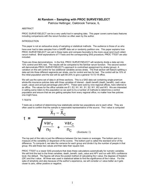
T-tests are a method of determining how statistically similar two populations are to each other. They are 

often used to confirm that the sample is reasonable representative of the source. The t value is computed 

(footnote 1) 

The top part of the ratio is just the difference between the two means or averages. The bottom part is a 

measure of the variability or dispersion of the scores. The bottom part is called the standard error of the 

difference. To compute it, we take the variance for each group and divide it by the number of people in that 

group. We add these two values and then take their square root. 

PROC TTEST is a newer SAS procedure that does these calculations automatically for numeric variables. 

We will limit the test to the three variables, death_benefit, cash_value and APY and run with 95% confidence 

level, the default. The figures will show the pooled method of calculating the t value, the degrees of freedom 

(DF) and the t value. All three was used in statistical tables to find the significance of the t-value. For the 

sake of simplicity and also because of the author’s experience, we will consider a t value better as it gets 

closer to zero, either positive or negative. 

1

10% CONTROL ACROSS THE ENTIRE POPULATION 

Our first try has us assigning control and test groups to our insurance population in a data set called 

single_prem_life. We will set up PROC SURVEYSELECT to assign 10% control and 90% across the entire 

data set. To obtain a reproducible sample, we will use the seed 828756043 instead of the default date and 

time to give a starting point for the selection: 

PROC SURVEYSELECT data=insur.single_prem_life outall seed=828756043 out=SFILE samprate=0.1; 

The insur.single_prem_life is the source data set, outall tells SURVEYSELECT to keep all of the 

observations in the output work data set SFILE and samprate=0.1 says to take 10% as the control. 

Our initial data set’s observation count was 104,722. All the original records are still in the output data set 

SFILE, so SFILE has the same number of observations. However SFILE will have three new variables 

added, samplingweight, selectionprob and most important from our point of view, selected. Selected is 

a Boolean variable, only available if you used the outall option. If 1, the observation was selected for the 

10%, if 0, it wasn’t. When we do a frequency on selected, we will see the 90-10 split as shown in Figure 1. 

Selected Frequency Percent Cumulative Frequency Cumulative Percent 

0 94249 90.00 94249 90.00 

1 10473 10.00 104722 100.00 

Figure 1 

To check whether our sample is representative, we can use PROC T-TEST with selected as the class 

variable. Note that any variable you use as the CLASS must have exactly two different values. 

PROC TTEST data=SFILE; 

Class selected; 

The Pooled method t values for our three variables of interest, death_benefit, cash_value and APY are in 

Figure 2: 

variable Name Method Variances DF t value 

death_benefit Pooled Equal 104720 1.26 

cash_value Pooled Equal 104720 -0.70 

APY Pooled Equal 104720 0.49 

Figure 2 

The ranuni method might use the code below to get the equivalent output. Our parameter to ranuni will be 

the same seed as the previous PROC SURVEYSELECT used: 

DATA SFILE; 

Rand=ranuni(828756043); 

Set insur.single_prem_life; 

If rand le .1 then selected=1; 

Else selected = 0; 

The frequencies in Figure 3 show a slightly different split: 

Selected Frequency Percent Cumulative Frequency Cumulative Percent 

0 94107 89.86 94107 89.86 

1 10615 10.14 104722 100.00 

Figure 3 

2

Our t values seem to be a little worse for the death_benefit and cash_value and a little worse for the APY: 

Variable Name Method Variances DF t value 

death_benefit Pooled Equal 104720 -1.52 


APY Pooled Equal 104720 -0.74 

Figure 4 

SAMPLING BY STRATA 

Where PROC SURVEYSELECT can really excel is when samples by group (strata) are needed. This works 

best if the source data is actually sorted by your strata variable(s). You can use the NOTSORTED option 

which might work if the data set is actually grouped by that variable, whether in order or not. Otherwise 

PROC SURVEYSELECT might take the entire group. It might even hang your session, depending upon the 

data structure. In Figure 5, the insur.single_prem_lifedata set, the data is not grouped by office, variable 

office. A 10% sample would probably take every observation. If grouped together like Figure 5B, we would 

get just 1 of each (Figure 6): 

Office death_benefit cash_value APY 

N1 50000 5000 3.99 

S1 70000 7000 4.15 

N1 50000 5000 3.99 

S1 70000 7000 4.15 

N1 50000 5000 3.99 

S1 70000 7000 4.15 

N1 50000 5000 3.99 

S1 70000 7000 4.15 

N1 50000 5000 3.99 

S1 70000 7000 4.15 

N1 50000 5000 3.99 

S1 70000 7000 4.15 

N1 50000 5000 3.99 

S1 70000 7000 4.15 

N1 50000 5000 3.99 

S1 70000 7000 4.15 

N1 50000 5000 3.99 

S1 70000 7000 4.15 

N1 50000 5000 3.99 

S1 70000 7000 4.15 

Figure 5 

3

Office death_benefit cash_value APY 

N1 50000 5000 3.99 

N1 50000 5000 3.99 

N1 50000 5000 3.99 

N1 50000 5000 3.99 

N1 50000 5000 3.99 

N1 50000 5000 3.99 

N1 50000 5000 3.99 

N1 50000 5000 3.99 

N1 50000 5000 3.99 

N1 50000 5000 3.99 

S1 70000 7000 4.15 

S1 70000 7000 4.15 

S1 70000 7000 4.15 

S1 70000 7000 4.15 

S1 70000 7000 4.15 

S1 70000 7000 4.15 

S1 70000 5000 4.15 

S1 70000 7000 4.15 

S1 70000 7000 4.15 

S1 70000 7000 4.15 

Figure 5B 

End sample: 

N1 50000 5000 3.99 

S1 70000 7000 4.15 

Figure 6 

It would definitely be a good idea to sort first. 

PROC SORT data= insur.single_prem_life out=policy_sorted; 

By office; 

And then use PROC SURVEYSELECT to take samples by office: 

PROC SURVEYSELECT data =policy sorted outall seed=828756043 out=SFILE samprate=.1; 

strata office; 

The strata statement tells SURVEYSELECT to take samples by office which must be sorted (default). 

The overall T-Test in figure 7 is a little different again from our first example 



cash_value Pooled Equal 104720 0.88 


Figure 7 

4

But this might be considerably different for each office as the T-Test in figure 8 demonstrates: 

Office variable Name Method Variances Office DF 

Office t 

value 

E1 death_benefit Pooled Equal 33772 -0.30 






N1 death_benefit Pooled Equal 20 0.94 






S1 death_benefit Pooled Equal 9077 0.59 






W1 death_benefit Pooled Equal 16 . 


APY Pooled Equal 16 . 

W2 death_benefit Pooled Equal 49 -2.94 



W3 death_benefit Pooled Equal 37948 1.46 



Figure 8 

5

We still have our 10% overall as shown by Figure 9. However, the number of policies per offices is 

considerably different. We might not be able to get a good test for those from the N1, W1 and W2 samples 

due to their low volumes (figure 9B): 

Selected Frequency Percent 

Cumulative 

Frequency 

Cumulative 

Percent 

0 94246 90.00 94246 90.00 

1 10476 10.00 104722 100.00 

Figure 9 

OFFICE SELECTED Frequency Percent 

Cumulative 

Frequency 

Cumulative 

Percent 

E1 0 30396 90.00 30396 90.00 

E1 1 3378 10.00 33774 100.00 

E2 0 108 90.00 108 90.00 

E2 1 12 10.00 120 100.00 

N1 0 19 86.36 19 86.36 

N1 1 3 13.64 22 100.00 

N2 0 20430 90.00 20430 90.00 

N2 1 2271 10.00 22701 100.00 

S1 0 8171 90.00 8171 90.00 

S1 1 908 10.00 9079 100.00 

S2 0 906 89.97 906 89.97 

S2 1 101 10.03 1007 100.00 

W1 0 16 88.89 16 88.89 

W1 1 2 11.11 18 100.00 

W2 0 45 88.24 45 88.24 

W2 1 6 11.76 51 100.00 

W3 0 34155 90.00 34155 90.00 

W3 1 3795 10.00 37950 100.00 

Figure 9B 

6

A comparison of the final distribution between PROC SURVEYSELECT without strata, ranuni and PROC 

SURVEYSELECT with strata (office) is in figure 10. Note that we didn’t get any at all for W1, using ranuni: 

FREQ 

10% 

SURVEY 

SELECT 

w/o 

Strata 

PCT 

10% 

SURVEY 

SELECT 

w/o 

Strata 

FREQ 

10% 

Ranuni 

PCT 

Ranuni 

Overall 

FREQ 

10% 

SURVEY 

SELECT 

w/ Strata 

PCT 

10% 

SURVEY 

SELECT 

w/ Strata 

OFFICE SELECTED 

E1 0 30388 89.97 30338 89.83 30396 90.00 

E1 1 3386 10.03 3436 10.17 3378 10.00 

E2 0 105 87.50 107 89.17 108 90.00 

E2 1 15 12.50 13 10.83 12 10.00 

N1 0 21 95.45 20 90.91 19 86.36 

N1 1 1 4.55 2 9.09 3 13.64 

N2 0 20445 90.06 20438 90.03 20430 90.00 

N2 1 2256 9.94 2263 9.97 2271 10.00 

S1 0 8197 90.29 8143 89.69 8171 90.00 

S1 1 882 9.71 936 10.31 908 10.00 

S2 0 911 90.47 897 89.08 906 89.97 

S2 1 96 9.53 110 10.92 101 10.03 

W1 0 17 94.44 18 100.00 16 88.89 

W1 1 1 5.56 0 0.00 2 11.11 

W2 0 46 90.20 45 88.24 45 88.24 

W2 1 5 9.80 6 11.76 6 11.76 

W3 0 34119 89.91 34101 89.86 34155 90.00 

W3 1 3831 10.09 3849 10.14 3795 10.00 

Figure 10 

7

The T-test comparison is shown in Figure 11. We can’t run a t-test for ranuni’s W1 observations because 

there is only value for selected: 0. 

10% 

SURVEY 

SELECT 

w/o 

Strata 

10% 

SURVEY 

SELECT 

w/ Strata 

10% 

Office variable Name Method Variances DF 

Ranuni 

E1 death_benefit Pooled Equal 33772 1.91 -2.21 -0.30 

cash_value Pooled Equal 33772 -0.68 -0.86 0.22 

APY Pooled Equal 33772 -0.20 -0.36 0.25 

E2 death_benefit Pooled Equal 118 -3.79 1.13 -0.64 

cash_value Pooled Equal 118 0.18 0.77 0.33 

APY Pooled Equal 118 1.02 0.94 0.90 

N1 death_benefit Pooled Equal 20 0.19 -0.09 0.94 



N2 death_benefit Pooled Equal 22699 -2.17 0.37 2.39 

cash_value Pooled Equal 22699 0.06 -1.56 1.34 

APY Pooled Equal 22699 0.18 -0.63 1.15 

S1 death_benefit Pooled Equal 9077 1.84 -0.27 0.59 



S2 death_benefit Pooled Equal 1005 0.50 0.23 0.92 

cash_value Pooled Equal 1005 0.71 -0.37 0.36 


W1 death_benefit Pooled Equal 16 . . 

cash_value Pooled Equal 16 -0.02 0.41 

APY Pooled Equal 16 . . 

W2 death_benefit Pooled Equal 49 0.33 0.36 -2.94 

cash_value Pooled Equal 49 -2.31 0.12 -0.31 

APY Pooled Equal 49 0.68 0.75 -0.92 

W3 death_benefit Pooled Equal 37948 0.56 -0.23 1.46 

cash_value Pooled Equal 37948 -1.06 -1.29 -0.05 


Figure 11 

If the company wanted to merge offices, this distribution might aid in that decision. For the purpose of this 

paper though, we will leave them as is. 

Suppose we wanted to adjust the sample size taken from each stratum. We might want everything from N2, 

S1, W1 and W2 so we could write our proc to take 100% from those strata. We know there are nine of them 

so we can write a statement like this: 

PROC SURVEYSELECT DATA=insur.single_prem_life outall seed=828756043 out=SFILE samprate=( 0.1, 

0.1, 0.1, 1.0, 1.0, 0.1, 1.0, 1.0, 0.1); 

Strata office; 

8

Or we could specify the sample size as actual numbers and add the selectall option to take all the 

observations in an office in case we don’t have enough to make up the count. This can be seen with the 

value 60 for office W2 which does not have enough observations to fulfill the request. 

PROC SURVEYSELECT data=insur.single_prem_life selectall outall seed=828756043 out=SFILE 

sampsize= (908, 101, 3378, 20, 22, 2271, 18, 60, 3795); 


It’s easy to lose track of these strata – if you end up with too many or too few in the samprate or sampsize 

parameter, you will get an error. A better way might be to keep your parameters in a data set. The example 

below loads a SAS data set with office, _rate_ and _nsize_ . Any variables besides _rate_ and _nsize_ 

must be present as named in the source data set or you will get unpredictable results. The _rate_ variable 

is required if using the samplepct data set with the samprate parameter and the _nsize_ with sampsize: 

DATA samplepct: 

attrib office format=$2. _rate_ format=6.3 _NSIZE_ format=6.; 

office='E1'; _nsize_=908; _rate_=0.1; output; 

office='E2'; _nsize_=101; _rate_=0.1; output; 

office='N1'; _nsize_=3378; _rate_=0.1; output; 

office='N2'; _nsize_=20; _rate_=1.0; output; 

office='S1'; _nsize_=22; _rate_=1.0; output; 

office='S2'; _nsize_=2271; _rate_=0.1; output; 

office='W1'; _nsize_=18; _rate_=1.0; output; 



Now, PROC SURVEYSELECT will take a sample of every stratum that matches the list. The SAS log should 

warn of any that do not. Here is how you would use the list for sampling rate: 

PROC SURVEYSELECT data=insur.single_prem_life outall seed=828756043 out=SFILE 

samprate=samplepct; 

strata office; 

You would replace the samprate statement with sampsize for sampling by size: 

PROC SURVEYSELECT data=insur.single_prem_life outall seed=828756043 out=SFILE 

sampsize=samplesize; 

Run; 

The good thing about using a data set for either your sample rate or sample size is that you will get output 

even if one or more of your strata change or perhaps disappear altogether (W1 and W2 taken over by W3?). 

However for any new strata values not in your list, you will get a warning in your log that there wasn’t any 

match. The step continues but nothing will be output for that stratum even with the OUTALL option. 

CONTROLLING FOR CERTAIN VARIABLES 

We might want to control for death benefit and cash value since these are of special interest. To use 

controls, the sampling method cannot be the default simple random method we did before. We will use 

another method, systemic random selection instead. The stratum is sorted by the control variables, a 

starting point is chosen at random from the sampling stratum, and thereafter at regular intervals. Since our 

control variables are death benefit and cash value, the sample will be taken from a random start in each 

office and then at regular intervals within death benefit and cash value. Unlike the strata, the source data 

set doesn’t need to be sorted by the control variables first. Notice the two additions we made to the request. 

One is specifying the method =SYS and the other is the CONTROL statement:. 

9

PROC SURVEYSELECT data=insur.single_prem_life outall method=sys seed=828756043 out=SFILE 

samprate=0.1; 


control death_benefit cash_value; 

Run; 

Overall the T-Test has better t values for these two variables: 





Figure 12 

It seems most of our offices t values also became closer to zero: 

Office variable Name Method Variances Office DF 

Office t 

value 

E1 death_benefit Pooled Equal 33772 0.28 



E2 death_benefit Pooled Equal 118 0.19 



N1 death_benefit Pooled Equal 20 -0.24 



N2 death_benefit Pooled Equal 22699 -0.39 



S1 death_benefit Pooled Equal 9077 -0.59 















Figure 13 

10

DESIGNING A CONTROL AND TWO TEST POPULATIONS 

We can do this with two PROC SURVEYSELECT steps. First we'll take just the 10% control. We'll then 

split the output into two data sets, control and test. PROC SURVEYSELECT against the test population will 

select an additional 20%. The last step puts the output data sets together for the final population. 

10% control 

Sort the data by office, then use PROC SURVEYSELECT to take a 10% sample by office. Output all 

records: 

PROC SURVEYSELECT data =policy_sorted outall seed=828756043 out=control_test samprate=0.1; 


The T-Test looks like this overall: 





Figure 14 

By office: 

Office variable Name Method Variances Office DF Office t value 






















W2 death_benefit Pooled Equal 49 -2.94 






Figure 15 

11

But now split the output into test and control. The control group is indicated by having its selected variable 

reset to 2. We also created a control_ind variable: 

DATA test_group control_group; 

set control_test; 

if selected eq 1 then do; 

selected=2; control_ind='C'; output control_group; 

else do; 

control_ind='T'; output test_group; 

end; 

Sort the test_group by office and take 20% again. Output everything to test_group2: 

PROC SURVEYSELECT data =test_group outall seed=828756043 out=test_group2 samprate=.2; 


We can run a T-Test again comparing the 20% test to the 80%. Overall, this is: 





Figure 16 

12

By office: 

Office variable Name Method Variances 

Office 

DF 

Office t 

value 
















S2 death_benefit Pooled Equal 904 -2.54 












Figure 17 

Then put the control group and test groups together and assign a population code (POP_CODE): 

data final_pop; 

set control_group(in=a) test_group2(in=b); 

if selected eq 2 then POP_CODE = 'CONTROL'; 

else if b and selected = 0 then POP_CODE='TEST1 '; 

else if b and selected =1 then POP_CODE='TEST2 '; 

13

A cross-tab by control indicator and population code overall gives us this: 

CONTROL_IND POP_CODE FREQUENCY PERCENT 

CUMULATIVE 

FREQUENCY 

C CONTROL 10476 10.00 10476 

T TEST1 75393 71.99 85869 

T TEST2 18853 18.00 104722 

Figure 18 

By office: 

OFFICE CONTROL_IND POP_CODE FREQUENCY PERCENT 

CUMULATIVE 

FREQUENCY 

E1 C CONTROL 3378 10.00 3378 

T TEST1 24316 72.00 27694 

T TEST2 6080 18.00 33774 

E2 C CONTROL 12 10.00 12 

T TEST1 86 71.67 98 

T TEST2 22 18.33 120 

N1 C CONTROL 3 13.64 3 

T TEST1 15 68.18 18 

T TEST2 4 18.18 22 

N2 C CONTROL 2271 10.00 2271 

T TEST1 16344 72.00 18615 

T TEST2 4086 18.00 22701 

S1 C CONTROL 908 10.00 908 

T TEST1 6536 71.99 7444 

T TEST2 1635 18.01 9079 

S2 C CONTROL 101 10.03 101 

T TEST1 724 71.90 825 

T TEST2 182 18.07 1007 

W1 C CONTROL 2 11.11 2 

T TEST1 12 66.67 14 

T TEST2 4 22.22 18 

W2 C CONTROL 6 11.76 6 

T TEST1 36 70.59 42 

T TEST2 9 17.65 51 

W3 C CONTROL 3795 10.00 3795 

T TEST1 27324 72.00 31119 

T TEST2 6831 18.00 37950 

Figure 19 

OTHER PROC SURVEYSELECT OPTIONS AND STATEMENTS 

ID var1 var2, etc. - Not only can you choose whether to output all the observations but the id statement lets 

you direct which variables to output. 

Noprint – do not print the output – output is nominal and will contain the sampling method, the seed, the 

number of samples selected, the strata variable (if any) and the number of strata. 

Nmin and nmax. These are used with the samprate= option to give a minimum and maximum amount of 

observations. This is the only the selectall option can be used with the samprate option. You may want 

20% but no more than 500 observations (nmax). Or still 20% but at least 500 or all of them if 500 can’t be 

found (nmin). 

14

CONCLUSION 

PROC SURVEYSELECT is a very useful procedure for sampling that seems to give at least as accurate 

results as the older ranuni method. In addition, you will find the performance for taking samples from a very 

large data set (remove the OUTALL option) is much better because PROC SURVEYSELECT does not have 

to read the entire source data set. 

FOOTNOTES 

Footnote 1 – T-Test mathematical equation and explanation taken from Research Methods Knowledge Base 

web site section on T-tests. 

ACKNOWLEDGEMENTS 

Thanks to Joe and Paul Butkovich for your encouragement and support. 

CONTACT INFORMATION 

Your comments and questions are valued and encouraged. The author is often on the road but can be 

contacted at 

Patricia Hettinger 

Email: patricia_hettinger@att.net 

Phone: 331-462-2142 

SAS and all other SAS Institute Inc. product or service names are registered trademarks or trademarks of 

SAS Institute Inc. in the USA and other countries. ® indicates USA registration. 

Other brand and product names are trademarks of their respective companies. 

15

At Random â Sampling with PROC SURVEYSELECT

Create successful ePaper yourself

Delete template?

Save as template?

At Random â Sampling with PROC SURVEYSELECT