Risk-Based Portfolio Optimization Using SAS Wei Chen, SAS ...

Risk-Based Portfolio Optimization Using SAS ®
Wei Chen, SAS Institute Inc., Cary, NC
ABSTRACT
In the midst of the recent turbulence in financial markets, risk management has become an increasingly critical part of
the decision-making process in financial institutions. A risk-based profitability strategy helps increase firm value and
helps avoid costs associated with financial distress. This paper explains how advanced risk analysis and optimization
products from SAS® can work together to enable optimal, risk-adjusted portfolio decisions. Several portfolio
optimization problems are discussed: (1) maximization of portfolio return subject to a target risk tolerance, expressed
as standard risk measures such as value at risk (VaR); (2) minimization of asset/liability mismatch through cash flow
allocation minimization; and (3) minimization of capital requirements by employment of an optimal risk mitigation
strategy. For these problems, best-practice solutions are presented using SAS Risk Management solutions.
INTRODUCTION
Modern financial theory has supported a strong relationship between profitability and risk. Risk borne by an
investment should be compensated by excess return. Financial institutions such as banks are known to take the risk
intermediation function for the entire economy. Adequate recognition of the underlying risk of an investment strategy
is a critical part of a financial decision process. Markowitz (1952) introduced the seminal risk-based portfolio
optimization model, which won him the 1990 Nobel Prize for Economics, together with William Sharpe and Merton
Miller. (All three laureates were awarded the Nobel Prize for their work in risk-based decision theories in investment
and corporate finance.)
The past few decades have seen tremendous advances in financial markets. The innovations of financial products
and financial management tools have contributed many good aspects to economic development. The complication in
the financial market has made both researchers and practitioners realize the limitation of the normality assumption in
the earlier work of the risk portfolio theory. In the early 1990s, J. P. Morgan proposed a new risk measure, value at
risk (VaR), which is a possible loss or value at a certain confidence interval. Statistically, VaR is simply a percentile
of a distribution. It extends the standard deviation to a measure that does not restrict its application to the normal
distribution. Other risk measures have been proposed as alternatives to standard deviation and VaR in the last
decade. Artzner et al. (1997) summarized the fundamental properties of a coherent risk measure. Based on these
new risk measures, the Basel committee proposed two international regulatory capital requirements in 1988 and
2004, known as Basel I and Basel II (Basel Committee 1988 and Basel Committee 2004). Following suit, the
European Commission has recently published the new, risk-based capital requirement framework known as Solvency
II (European Commission 2008) for insurance companies. With the emergence of the new risk measures and riskbased
capital requirement, Markowitz’s risk-based portfolio optimization framework can be extended to robust forms.
The technique of portfolio optimization is not only useful for portfolio selection, it is also useful in areas like asset
pricing, collateral allocation, and asset liability management. The basic idea is to apply risk measures in an optimal
decision process.
Three categories of single-stage optimization approaches are typically seen for portfolios with stochastic nature: (1)
reduced form—risk statistics for example standard deviation, risk weights are estimated separately from the
optimization problem; (2) stochastic programming—risk is explicitly modeled in an optimization process; and (3)
simulation-based optimization—optimization over a simulated sample space that turns stochastic programming into a
deterministic programming problem. This paper presents several implementations of risk-based portfolio optimization
using SAS Risk Management solutions that leverage SAS risk computation and optimization procedures. With the
strong portfolio simulation power in SAS Risk Management solutions, all of the optimizations covered in this paper
have an approach. “A Brief Review of Risk Measures” explains a few risk measures and portfolio optimization
business cases. “Portfolio Optimization” introduces portfolio optimization that is used in portfolio selection. “Asset
Liability Management with Stochastic Cash Flow” extends portfolio optimization to a cash-flow-based decision
environment. “Optimal Credit Risk Mitigant Allocation” introduces an innovative optimal credit risk mitigant allocation
algorithm in a credit risk portfolio under the new Basel II regulatory capital requirement framework. “Conclusion”
concludes the paper.
A BRIEF REVIEW OF RISK MEASURES
For two portfolios—X and Y—Artzner et al. (1997) prescribed the following conditions for a risk measure m to be
COHERENT:
1

• Subadditivity – m X + Y ≤ m X + m(Y): diversification is good for a portfolio.
• Homogeneity – m tX = tm X for any constant t: no scale effect on a portfolio risk.
• Monotonicity – m(X) ≥ m(Y) if X>Y almost surely: risk is duely reflected in the risk measure.
• Translation invariance – m X + r = m X + r: risk-free asset does not contribute to overall risk.
Coherence of a risk measure is important for many reasons. Subadditivity and monotonicity together implies
convexity, which is a necessary condition for the existence of a global optimum. A well-known result documented by
Artzner et al. (1997) is that the widely accepted VaR measure introduced below is not guaranteed to be a coherent
risk measure unless the underlying risk distribution belongs to an elliptic family.
The following risk measures are widely used in financial risk management:
Standard Deviation: It is mostly used as a statistical measure to describe the volatility of random variables.
In a nonparametric setting, the measure is defined as:
σ = E[X − E X ] 2 ,
where E stands for the expectation of a random variable. In practice, people use the standard error from a
sample space as an estimator of the standard deviation.
The standard deviation captures the randomness of a normally distributed risk variable. It is also a
coherence risk measure for most of the early work of the modern finance theory, including Markowitz’s
portfolio optimization, Sharpe (1964)’s capital asset pricing model (CAPM), and Black and Scholes (1973)’s
option pricing formula. Only for elliptic-distributed underlying risk volatility, VaR , and expected shortfall are
all equivalent because of the scalability of these distributions. For example, for normal distribution, VaR is
simply a multiple of the standard deviation, where the multiplier is the corresponding percentile on a
standard normal distribution.
VaR: It has been a widely used measure in risk management since its birth. In simple business terms, it
represents the maximum value or loss at a given confidence interval. Mathematically, it is defined as:
VaR α = inf⁡[x|P(X ≥ x) ≥ α],
where α is the given confidence interval. It is usually estimated in the same way as a percentile of a
distribution for the given confidence interval α.
VaR works for all distribution assumptions and provides intuitive business justification. As a result, it is used
by many financial institutions despite its unwarranted coherence in general.
Expected Shortfall (or Conditional VaR): It is a coherent risk measure. By definition, it is:
ES α = E[X|X ≥ VaR α ]
where VaR α is the VaR previously defined. For a fat tail distribution, expected shortfall is not guaranteed
to exist. If it exists, it represents the expected value or loss beyond a given confidence interval. For a given
sample space, expected shortfall is estimated as the mean of the points beyond and including VaR of a
confidence interval α. This conditional mean calculation requires caution to remain convex.
SAS Risk Management solutions compute these risk measures and their variations using standard statistical
algorithms.
An important application of these risk measures is to calibrate a financial institution’s capital requirement. Such
capital is a financial institution’s own funds that are set aside to protect the institution from insolvency from big losses.
This capital is oftentimes required to cover projected unexpected loss of a given confidence interval, which makes a
connection to the risk measures. For example, the Basel II capital requirement for banks is based on 99% VaR for
market risk (internal model approach) and 99.9% VaR for credit risk.
PORTFOLIO OPTIMIZATION
Portfolio optimization has wide applications in portfolio asset allocation and asset pricing. The traditional portfolio
optimization is mean-variance optimization, which was originated by Markowitz (1952). The decision rule is to
maximize the expected return of the portfolio, while keeping the return variance to a certain level. (Or to minimize the
2

eturn variance for a given expected return.) The resulting portfolios for different desired variance levels make a socalled
mean-variance efficient frontier. Mean-variance optimization led to the birth of CAPM, which was introduced
by Sharpe (1964). In the following sections, mean-variance, mean-expected-shortfall (mean-ES), and mean-value-atrisk
(mean-VaR) optimizations (supported in the SAS Risk Dimensions OPTIMIZATON statement) are explained.
MEAN-VARIANCE OPTIMIZATION
Let θ = (θ 1 , … , θ M ) be a vector of random returns of M assets in a portfolio.
Let x = (x 1 , … , x M )′ be a vector of the percentage of the portfolio invested in these assets.
The expected returns vector is θ. The covariance matrix of returns on these M assets is Q. The mean-variance
optimization seeks to find an optimal vector x such that:
(1) max x x′θ
is subject to:
x ′ Qx ≤ δ 2
M
i=1
x i = 1
lb ≤ x ≤ ub,
where δ 2 is a preset tolerance of the variance of portfolio return, lb and ub are vectors of the lower and upper bounds
of percentage weight on the assets in the portfolio. A user can also add linear business constraints (for example,
weights on fixed-income assets in the portfolio retained at a certain level).
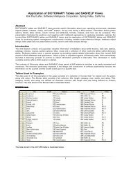
The optimal solutions to (1) from a range of δ 2 constraints result in a mean-variance efficient frontier. An example of
the mean-variance efficient frontier created by SAS Risk Dimensions for a sample portfolio is illustrated in figure 1. It
shows a portfolio of fixed incomes, derivatives, and equities based on a historical simulation over monthly interest
rates, foreign exchange rates, and equity prices data from August 1998 to August 2001. The range of volatility
constraint is (0, 0.03).
Figure 1. Mean-Variance Efficient Frontier of a Portfolio in an Historical Simulation
MEAN-ES AND MEAN-VAR OPTIMIZATIONS
Because of the limitation on volatility, mean-VaR optimization is becoming more popular in portfolio optimization.
Both VaR and expected shortfalls are related to set of percentiles on a return distribution. Because expected shortfall
is a convex risk measure, it is more amenable for global optimization than VaR and volatility. Let’s assume a
3

confidence interval α for the expected shortfall for the return distribution with density function p ∙ , which warrants a
finite expected return of the portfolio. (The analytical presentation turns out to be unimportant for the optimization
problem). Following the definition of expected shortfall and using the same notations as in (1), expected shortfall can
be expressed as the conditional expectation of the portfolio return associated with choice of asset weights x can be
expected as:
(2) φ α x, γ = γ + 1
−x ′ θ − γ + p θ dθ,
1−α
where γ is the smallest 1 solution to:
ω x, γ = I( − x′θ ≤ γ) p θ dθ = α, [y] + y, y > 0
= {
0, y ≤ 0
and I z = {1,
if z is true
0, otherwise .
Rockafellar and Uryasev (2000) proved that (2) is a convex and continuously differentiable function. They show that
in a sample space of N, simulated samples from the distribution of θ, can be further approximated by a convex (in
x, γ) and piecewise linear (in γ) function:
φ α x, γ = γ + 1 N
−x ′ θ j − γ +
(1−α)N j=1
Therefore, given a simulation with N scenarios, a mean-ES 2 optimization is equivalent to finding the solution for:
(3) min (x,γ) γ + 1 N z j
(1−α)N j =1
which is subject to:
x′θ ≥ μ
z j ≥ 0
x ′ θ j + γ + z j ≥ 0, for j = 1, … , K
M
i=1
x i = 1
lb ≤ x ≤ ub,
where μ is the preset target of mean return, and z j are the auxiliary variables that are derived from the simulated
distribution of N simulated scenarios.
Similar to (1), linear business constraints can be added to (3) as well. Based on the above idea, SAS Risk
Dimensions uses a scenario-based approach that converts a stochastic optimization into a deterministic optimization
with simulated scenarios.
A mean-VaR optimization can be expressed as the following:
(4) min x [V α,N (−x ′ θ 1 , … , −x ′ θ N )]
which is subject to:
x′θ ≥ μ
M
i=1
x i = 1
lb ≤ x ≤ ub.
VaR is not a convex risk measure for most of the non-elliptic distributions, so (4) might not warrant a well-behaved
optimization problem. However, Rockafellar and Uryasev (2000) have shown that from the presentation of the mean-
ES problem (3), it can be seen that γ is a lower bound to the VaR at confidence interval α. Therefore, one can
iteratively minimize (3) with respect to γ to approach the optimal solution of (4). On the other hand, a brute force
nonlinear optimization using PROC NLP is also accommodated in SAS Risk Dimensions.
VaR and expected shortfall minimization might not always be a well-posed problem, even if the convexity is satisfied.
Alexander et al. (2004) gave an example of an ill-posed optimization problem for a derivative portfolio where
derivatives are evaluated with the delta-gamma approximation. The linear programming of an expected-shortfallbased
approach becomes inefficient for a large portfolio in this case.
1 Equation ω x, γ = α might contain more than one solution, although ω x, γ is a continuous and non-decreasing function.
2 Krokhmal et al. (2002) showed that the mean-ES optimization in (3) generates the same efficient frontier as maximizing the
mean return subject to a preset tolerance of expected shortfall using the same auxiliary variable representation. Both
optimizations are supported in SAS Risk Dimensions.
4

More information about the implementation of the previous problems can be found in the documentation of the
OPTIMIZATION statement in SAS Risk Dimensions.
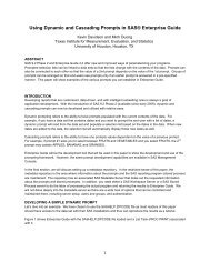
ASSET LIABILITY MANAGEMENT WITH STOCHASTIC CASH FLOW
Figure 2. Sample Asset Liability Gap for a Range of Time Buckets
The previous optimization cases were based on the market value of the positions in a financial institution’s portfolio.
A lot of financial business is cash-flow-based. As market intermediator, a bank typically borrows from and lends to
different finance sources and makes a profit from the process. A pension fund must produce income cash flow from
5

its investments to support its payout commitment. Similarly, an insurance company relies on income from its assets
and fees to cover its liabilities. For any institution with outstanding debts, enough cash flow from future business
operations is critical for the institution to keep a good credit status. In these cases, decisions have to be made based
on future cash flows generated from a portfolio of assets and liabilities. Ziemba (2003) has more details about the
optimization for asset liability management.
Cash flows from positions in a portfolio can happen on different dates and be of different amounts. To simplify the
cash flow analysis, financial institutions usually group cash flows into a set of predefined time buckets in the future.
The choice of time buckets is specific to each institution’s business strategy and operational life cycle. The bucketed
cash flows are compared by asset and liability. Any significant gaps between the two might call for an alternate
business strategy. There are many ways that gaps can be constructed. For example, one can compare the
scheduled single or accumulated cash flow amounts in each bucket to look for a potential liquidity problem, or one
can check the cash flows that are subject to rate adjustment (repricing) in future time periods, or one can compare
durations and convexities (both are sensitivity measures) of the cash flows. For a portfolio of fixed incomes and
derivatives across regions of London, New York, and Tokyo, figure 2 shows a portion of the cash flow gap report
produced by SAS Risk Dimensions and SAS Risk Management for Banking.
SAS Risk Management for Banking enables the user to leverage the strong cash flow analysis of PROC RISK and
the flexible optimization modeling of PROC OPTMODEL to accomplish decision objectives for asset and liability
management. The process involves the following steps:
1. Simulate market states based on user-specified simulation methods (model-based, historical, or scenario).
2. Generate cash flows of user-defined types (maturity, repricing, interest income, and so on) for each
simulated market state and collect them into buckets.
3. Analyze the bucketed cash flows by assets and liabilities (at each additional user-defined reporting
hierarchy).
4. Execute optimization based on a selected objective function and constraints for the cash flows.
This process is driven by data in SAS Risk Dimensions.
In general, the following optimization problem yields an institution’s asset allocation strategy to minimize the gap
between its asset and liability by maturity.
(5) min wt
f [
xA
tT
n
k1 iA,
jL
k k
( xiCt, i
Ct,
j
)]
Where:
A = a set of all instruments of which the positions can be adjusted.
L = a set of all fixed positions.
n = the number of simulated scenarios.
T = a set of time buckets.
x i = the number of shares of a particular asset instrument.
C t,i = the cash flow from either an asset or liability in time bucket t in a simulated scenario. Cash
flows from liability carry negative signs.
w t = the weight of a time bucket.
f ∙ the function that is determined by the decision rule.
This problem is subject to business constraints or risk (for example, VaR) constraints. Additional constraints might
include x i ≥ 0 if short-selling assets are not allowed. For the performance of the optimization, usually x i ’s are not
restricted to integers. In most cases, the function f(∙) is chosen as the least square or absolute function.
Equation (5) is a single-stage optimal portfolio allocation. A multi-stage problem would require dynamic portfolio
rebalance over the life of the decision process. Multi-stage optimization might be possible with a dynamic trading and
reinvestment feature that will soon be available in SAS Risk Dimensions.
A replicating portfolio has its roots in derivative pricing. The idea is to price a portfolio of illiquid assets with a set of
liquid assets that have tangible market values. The liquid assets must be able to replicate the cash flow streams of
the illiquid assets in all possible market scenarios. The recent birth of fair value rules has made the replicating
portfolio approach more important. For example, the Solvency II framework for European insurance and reinsurance
institutions has required the replicating portfolio technique to get the values of the insurance liabilities on the balance
sheet. The objective function for the replicating portfolio can be similar to the minimization problem (5), where
present values replace the straight values of all cash flows. That is, instead of C k t,i , the present value cash flow
6

discounted in the corresponding simulated scenario d k k
t C t,i is applied. Risk constraints like variance, expected
shortfall, and VaR can be applied to (5), which leads to a more risk-based replication. In the replicating portfolio
application, assets have to be chosen to represent the unique features in the underlying liability structure, including
optionality and payoff conditions. This topic is beyond the scope of this paper.
OPTIMAL CREDIT RISK MITIGANT ALLOCATION
Credit risk is one of the most significant risks a financial institution encounters every day. In general, credit risk is the
risk of loss induced by the failure of a counterparty to fulfill the contracted obligation. Financial institutions have
traditionally leveraged several tools such as guarantees, credit derivatives, collateral, or netting agreements to
mitigate losses due to credit risk. The well-specified credit mitigation tools are often recognized in the capital
requirement calculation. For example, Basel II has required the following:
Credit exposures must be risk-weighted based on their credit qualities.
If an eligible credit risk mitigant is present with an exposure, then the risk weight of the credit risk mitigant
can be used as the risk weight of the portion of the exposure that is covered by the credit risk mitigant.
The applicable value of the credit risk mitigant must be adjusted based on the nature of the mitigant.
Because an excessive capital level takes away an institution’s business development opportunity, it is to the benefit
of the institution to reduce its capital.
SAS introduced an optimal credit risk allocation method in its SAS Credit Risk Management for Banking solution
using the generalized network algorithm. Before the method is described, consider the concept of a generalized
network.
GENERALIZED NETWORK FOR AN EXPOSURE AND MITIGANT RELATION
Networks arise in numerous settings and in a variety of guises. Operations research has seen rapid advances in the
methodology and application of network optimization models. A network representation provides a powerful visual
and conceptual aid for portraying the relationships between the credit exposures and the credit risk mitigants. The
generalized network optimization model in this context poses a special type of linear programming problem that can
efficiently be solved with millions of exposures and mitigants that are in most banks.
Here are a few mathematical terms of the network models:
Node is an entity in the network usually labeled as suppliers, demanders, or transition.
Arc is the path from one entity to another.
Directed network is a network that has only directed arcs.
Arc cost is the cost associated with an arc when goods are moved from one end of the arc to the other.
Arc multiplier is the discount factor associated with an arc when goods move through it.
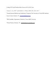
Figure 3 is a directed network representation of an exposure and mitigant network. There are three exposures—E1,
E2, and E3—and four credit risk mitigants—C1, C2, C3, and C4. The node NC supplies all of the unsecured portions
of the exposures in the diagram. The credit risk mitigants act as supply nodes and exposures act as demand nodes.
The flow costs are simply the risk weights associated with the mitigants. The arcs reflect the contractual relations
between credit risk mitigants and exposures. In figure 3, exposure E1 is secured by C1 and C2, E2 is secured by C3
only, and E3 is secured by C3 and C4. Any amount flowed out of the NC node takes the risk weight of the
correspondent exposure. The first number on each arc (exposure-mitigant relation) indicates the cost (risk weight)
associated with the arc.
To adjust for the potential changes in the material value of the credit risk mitigants, additional adjustments are
required based on the nature of the mitigants. For example, Basel II has required haircut discounts to financial
collaterals and nettings. In addition, if the exposures and credit risk mitigants are in different currencies, further
haircut discounts are required for the fluctuation of the foreign exchange rate dynamics. Because the discount might
depend on both the exposure and the credit risk mitigant, it is arc dependent. Using the generalized network model,
discounts can be added to the arc to represent the attrition in the goods. The second number on each arc indicates
the multiplier associated with the arc.
7

E1
0, 0.7
C1
[70]
50%, 1
[100]
200%, 1
C2
[60]
E2
0, 0.8
C3
[110]
300%, 1
[100]
0, 0.7
75%, 0.8
C4
E3
250%, 1
[150]
[200]
NC
Figure 3. Example of an Exposure Mitigant Network
OBJECTIVE FUNCTION
The regulatory credit risk capital requirement proposed by Basel II can be summarized as the computation of the
aggregated risk-weighted assets (which are a regulatory approximation of the VaR (previously introduced)):
(6)
RWA EAD RW i i
1
n
i
RWA stands for risk-weighted asset, EAD stands for exposure at default, and RW is the risk weight. The total
number of exposures is n. When credit risk mitigants are present with an exposure, the exposure can be
decomposed into an unsecured portion and several secured portions that take the adjusted value of the credit risk
mitigant. The secured portions take the risk weights that correspond to the mitigants. (Risk weight for a credit risk
mitigant does not necessarily have the same interpretation as the risk weight for an exposure, but it has a similar
effect.) The unsecured portion takes the risk weight of the exposure itself. The risk-weighted asset in equation (6)
can now be written as:
(7)
n
m
RWA ( SEC
i1 j 1
i
i
j
i
RW
j
i
USEC
RW )
i
i
SEC is the secured portion and USEC is the unsecured portion. Each exposure can be secured by several credit risk
mitigants. In general, multiple exposures covered by multiple credit risk mitigants should be considered in the
methodology description.
With the introduction of the arc multiplier, the regulatory capital is related to the following equation:
n mi
(8)
RWA ( SEC RW M USEC
RW )
i1 j 1
i
j
i
j
i
j
i
i
i
8

The optimal credit risk mitigant allocation for the objective function in the Basel II specification becomes a minimum
cost network flow problem with cost function (8).
The previous optimal credit risk mitigant allocation can be implemented using the
CRM_ALLOCATION_METHOD=”OPTIMAL” option in SAS Credit Risk Management.
AN EXAMPLE
Figure 3 further illustrates the problem and the proposed solution.
The Problem
A bank has three loan exposures—E1 through E3—and four credit risk mitigants—C1 through C4. Here is the
detailed information.
1. E1 has EAD $100 and is risk-weighted 200%. E2 has EAD $110 and is risk-weighted 300%. E3 has EAD
$200 and is risk-weighted 250%.
2. C1 and C3 are financial collaterals, C2 is a guarantee, and C4 is a receivable. C1 is worth $70. C2 is worth
$60 and is risk-weighted 50%. C3 is worth $100. C4 is worth $150 and is risk-weighted 75%.
3. The directed arcs in figure 3 represent the possible coverage between the credit risk mitigants and
exposures. They are typically specified by the business contracts and cannot be altered.
Financial collaterals are usually subject to haircut adjustments (collateral itself, and a currency mismatch adjustment,
if necessary). Let’s assume the haircut adjustments result in multipliers as (E1, C1)=0.7, (E2, C3)=0.8, and (E3,
C3)=0.7. The guarantee has no adjustment, so the multiplier on (E1, C2)=1. The receivable is subject to an overcollateralization
adjustment, which results in the multiplier (E3, C4)=0.8.
The regulatory capital requirement requires the risk-weighted asset to be calculated as equation (8). In addition, the
bank needs to report the risk weight for the secured and unsecured portions of each exposure.
The Solution
In this simple example, there are a few ways that the bank can apply the credit risk mitigants to the exposures.
1. For E1, there are two possible ways to apply the mitigants.
a. Apply C1 first and C2 second.
The secured portion by C1 is $49 with 0 risk weight. The secured portion by C2 is $51 with 50%
risk weight. The RWA for E1 is $25.50 (49*0+51*50%=25.5).
b. Apply C2 first and C1 second.
The secured portion by C2 is $60 with risk weight 50%. The secured portion by C1 is $40 with 0
risk weight. The RWA for E1 is $30 (60*50%+40*0=30).
2. E2 and E3 share C3, but E4 has sole claim to C4. There are two possible ways to apply the mitigants.
a. E2 is secured by C3 and E3 is secured by C4.
The secured portion of E2 by C3 is $80 with 0 risk weight. The unsecured portion is $30 with 300%
risk weight. The RWA for E2 is $90 (80*0+30*300%=90).
The secured portion of E3 by C4 is $120 with 75% risk weight. The unsecured portion is $80 with
250% risk weight. The RWA for E3 is $290 (120*75%+80*250%=290).
The total RWA for E2 and E3 is $380.
b. E3 is secured by C3 and C4. E2 is completely unsecured.
The secured portion of E3 by C3 is $70 with risk weight 0. The secured portion of E3 by C4 is $120
with risk weight 75%, which leaves $10 unsecured. The RWA for E3 is $185
(70*0+120*75%+10*250%=185). The RWA for E2 unsecured is $330 (110*300%=330).
The total RWA for E2 and E3 is $515.
Overall, there are four possible ways to apply the credit risk mitigants in this example. The optimal solution is the 1(a)
and 2(a) combination, where the total RWA is $405.5. The worst solution is the 1(b) and 2(b) combination, where the
total RWA is $545. For a bank with millions of exposures and credit risk mitigants, each worth hundreds of thousands
of dollars, the differences in the RWA because of mitigant allocations can be drastic. Having an optimal solution is
not trivial. SAS Credit Risk Management uses PROC OPTLP to solve this problem.
Because exposures and credit risk mitigants only form a closed network when they are related on the contractual
base, the minimal cost network optimization technique can be applied to each independent sub-network without
sacrificing the global optimum. In the above example, (E1, C1, C2) and (E2, E3, C3, C4) are two disjointed networks.
9

A network partition algorithm, based on the contractual relations between exposures and mitigants, is used in SAS
Credit Risk Management to recognize all of the sub-networks.
A point worth making is that the optimal allocation might not always be allowed if a business contract clearly states
how credit risk mitigants should be applied. SAS Credit Risk Management provides users with an option to honor the
contractual allocation, instead of the optimal allocation. Even if this is the case, the optimal allocation is still useful for
decision makers to get more insightful information on how risk can be reduced in an alternative way.
The generalized network approach to the optimal credit risk mitigant allocation provides an intuitive and efficient
algorithm to allocate exposures and credit risk mitigants to minimize credit risk. The objective function can be
extended beyond the Basel II capital requirement. When the problem extends with simulated scenarios, the variance,
VaR, and expected shortfall optimization techniques can be applied.
CONCLUSION
Risk-based portfolio optimization supports better financial decision making on a risk-adjusted basis. In a fluctuating
financial market, a risk-based decision process becomes more essential for a financial institution. This paper
presents several portfolio optimization methods in SAS Risk Management solutions that use risk modeling, analysis,
and optimization. These methods have many applications beyond financial portfolios. In a case where a decision
can be modeled with uncertainty (for example, a real option problem), a risk-based portfolio optimization can help
reach an intuitive result.
SAS Risk Management solutions strive to provide cutting edge solutions for decision making in a risk environment.
REFERENCES
Alexander, S., T. F. Coleman, and Y. Li. 2004, “Minimizing VaR and CvaR for a Portfolio of Derivatives.” Working
Paper, Cornell University, 2004.
Artzner, P., F. Delbaen, J. M. Eber, and D. Heath. 1997. “Coherent Measures of Risk.” Mathematical Finance 9:203-
228.
Black, F., and M. S. Scholes. 1973. “The Pricing of Options and Corporate Liabilities.” Journal of Political Economy
81(3):637-654.
Krokhmal, P., J. Palmquist, and S. Uryasev. 2002. “Portfolio Optimization with Conditional Value-at-Risk Objective
and Constraints.” Journal of Risk 4(2):43-68.
Markowitz, H. M. 1952. “Portfolio Selection.” Journal of Finance 7:77-99.
Rockafellar, R.T., and S. Uryasev. 2000. “Optimization of Conditional Value-at-Risk.” Journal of Risk 2(3):21-39.
Sharpe, W. F. 1964. “Capital asset prices: A theory of market equilibrium under conditions of risk.” Journal of Finance
19:425-442.
Ziemba, W.T. 2003. The Stochastic Programming Approach to Asset, Liability, and Wealth Management. Research
Foundation of CFA Institute.
RESOURCES
Basel Committee. 1988. International convergence of capital measurement and capital standards. Available at
http://www.bis.org/publ/bcbs04a.htm.
Basel Committee. 2004. Basel II: International Convergence of Capital Measurement and Capital Standards: a
Revised Framework. Available at http://www.bis.org/publ/bcbs107.htm.
Commission of the European Communities. 2008. Amended Proposal for a Directive of the European Parliament and
of the Council on the taking-up and pursuit of the business of Insurance and Reinsurance - (Solvency II). Available at
http://ec.europa.eu/internal_market/insurance/solvency/index_en.htm#proposal.
ACKNOWLEDGMENTS
The author is grateful to Donald Erdman and Jimmy Skoglund for their comments and suggestions.
10

CONTACT INFORMATION
Your comments and questions are valued and encouraged. Contact the author at:
Wei Chen
SAS Institute Inc.
SAS Campus Drive
Cary, NC 27513
E-mail: wei.chen@sas.com
SAS and all other SAS Institute Inc. product or service names are registered trademarks or trademarks of SAS
Institute Inc. in the USA and other countries. ® indicates USA registration.
Other brand and product names are trademarks of their respective companies.
11