SUN 20 NFE 009 EST - the School of Engineering and Applied ...
SUN 20 NFE 009 EST - the School of Engineering and Applied ...
SUN 20 NFE 009 EST - the School of Engineering and Applied ...

Create successful ePaper yourself
Turn your PDF publications into a flip-book with our unique Google optimized e-Paper software.
S<br />
<strong>SUN</strong>F<strong>EST</strong><br />
(www.seas.upenn.edu/~<br />
sunfest)<br />
T<br />
<strong>20</strong>09<br />
SUMMER UNDERGRADUATE FELLOWSHIPS<br />
IN<br />
SENSOR TECHNOLOGIES<br />
TECHNICAL REPORT<br />
TR-CST25AUG09<br />
Center for Sensor Technologies<br />
University<br />
<strong>of</strong> Pennsylvania<br />
Philadelphia, PA<br />
19104
Acknowledgement<br />
This material is based upon work supported by <strong>the</strong> National Science Foundation under Grant No. 0754741.<br />
Disclaimer<br />
Any opinions, findings, <strong>and</strong> conclusions or recommendations expressed in this material are those <strong>of</strong> <strong>the</strong> author(s)<br />
<strong>and</strong> do not necessarily reflect <strong>the</strong> views <strong>of</strong> <strong>the</strong> National Science Foundation.
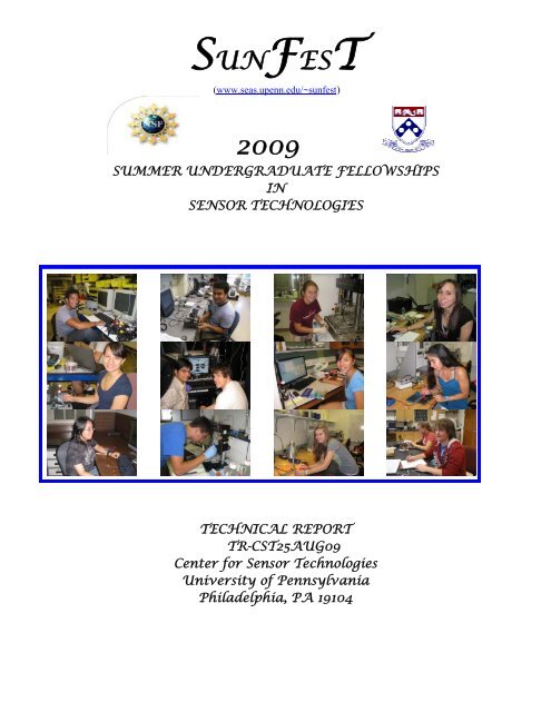
<strong>SUN</strong>F<strong>EST</strong> <strong>20</strong>09
<strong>SUN</strong>F<strong>EST</strong> <strong>20</strong>09<br />
SUMMER UNDERGRADUATE FELLOWSHIP IN SENSOR TECHNOLOGIES<br />
Sponsored by <strong>the</strong> National Science Foundation (Award no. EEC-0754741)<br />
PREFACE<br />
This report is <strong>the</strong> result <strong>of</strong> twelve undergraduate students’ research efforts during <strong>the</strong> summer <strong>of</strong><br />
<strong>20</strong>09; from June 1 through August 8, <strong>20</strong>09. Twelve students from Penn <strong>and</strong> o<strong>the</strong>r colleges participated<br />
in <strong>the</strong> <strong>SUN</strong>F<strong>EST</strong> program, which is organized by <strong>the</strong> Center for Sensor Technologies <strong>of</strong> <strong>the</strong> <strong>School</strong> <strong>of</strong><br />
<strong>Engineering</strong> <strong>and</strong> <strong>Applied</strong> Science at <strong>the</strong> University <strong>of</strong> Pennsylvania. This unique “Summer Experience for<br />
Undergraduates in Sensor Technologies” program was initiated in 1986 <strong>and</strong> has grown considerably in<br />
size. It is now recognized as one <strong>of</strong> <strong>the</strong> most successful summer programs for undergraduates in <strong>the</strong><br />
country. I would like to express my sincere gratitude to <strong>the</strong> National Science Foundation for <strong>the</strong>ir<br />
continued support for this REU Site.<br />
The purpose <strong>of</strong> <strong>the</strong> <strong>SUN</strong>F<strong>EST</strong> program is to provide bright, motivated undergraduate students with<br />
<strong>the</strong> opportunity to become involved in active research projects under <strong>the</strong> supervision <strong>of</strong> a faculty<br />
member <strong>and</strong> his graduate student(s). The general area <strong>of</strong> research concentrates on sensor<br />
technologies <strong>and</strong> includes projects such as materials <strong>and</strong> technology for sensors, microstructures,<br />
smart imagers, bio-sensors <strong>and</strong> robotics. By providing <strong>the</strong> students with h<strong>and</strong>s-on experience <strong>and</strong><br />
integrating <strong>the</strong>m with a larger research group where <strong>the</strong>y can work toge<strong>the</strong>r with o<strong>the</strong>r students,<br />
<strong>the</strong> program intends to guide <strong>the</strong>m in <strong>the</strong>ir career choices. By exposing <strong>the</strong> students to <strong>the</strong> world <strong>of</strong><br />
research, we hope <strong>the</strong>y will be more inclined to go on for advanced degrees in science <strong>and</strong><br />
engineering.<br />
The students participated in a variety <strong>of</strong> h<strong>and</strong>s-on workshops in order to give <strong>the</strong>m <strong>the</strong> tools to do<br />
first-rate research or enhance <strong>the</strong>ir communication skills. These included “Ethics in Science <strong>and</strong><br />
<strong>Engineering</strong>”, “Information Retrieval <strong>and</strong> Evaluation”, “Applying to Graduate <strong>School</strong>” <strong>and</strong> “Writing<br />
Technical Reports”. Students also had plenty <strong>of</strong> opportunity for social interactions among <strong>the</strong>mselves or<br />
with faculty <strong>and</strong> graduate student advisors.<br />
This booklet contains reports from this year’s projects, <strong>the</strong> quality <strong>of</strong> which testifies to <strong>the</strong><br />
high level <strong>of</strong> research <strong>and</strong> commitment by <strong>the</strong>se students <strong>and</strong> <strong>the</strong>ir supervisors. I would like<br />
to express my sincere thanks to <strong>the</strong> students for <strong>the</strong>ir enthusiastic participation; <strong>the</strong> help <strong>of</strong><br />
<strong>the</strong> faculty members, graduate students <strong>and</strong> support staff is very much appreciated. I would<br />
also like to thank Sherri Butler, Delores Magobet, Valerie Lundy-Wagner, Sid Deliwala, <strong>and</strong><br />
<strong>the</strong> rest <strong>of</strong> <strong>the</strong> ESE staff for <strong>the</strong>ir invaluable help in making this program run smoothly.<br />
Jan Van der Spiegel, Director<br />
Center for Sensor Technologies<br />
i
FINAL REPORT<br />
<strong>20</strong>09 SUMMER UNDERGRADUATE FELLOWSHIP IN SENSOR TECHNOLOGIES<br />
Sponsored by <strong>the</strong> National Science Foundation<br />
http://www.ese.upenn.edu/~sunfest/pastProjects/Projects09.html<br />
TABLE OF CONTENTS<br />
PREFACE <strong>and</strong> LIST OF STUDENT PARTICIPANTS<br />
DESIGN OF A SYSTEM TO STUDY HUMAN INTERNAL DISC STRAINS IN<br />
TORSION AND COMPRESSION MEASURED NONINVASIVELY USING MAGNETIC<br />
RESONANCE IMAGING<br />
Valerie, Walters (ESM) – Virginia Polytechnic Institute <strong>and</strong> State University<br />
Advisor: Dawn M. Elliot, PhD<br />
AMPLIFICATION CIRCUITS AND PATTERNING METHODS OF ORGANIC FIELD-<br />
EFFECT TRANSISTORS<br />
Hank Bink (Electrical <strong>and</strong> Computer <strong>Engineering</strong>) – Lafayette College<br />
Advisor: Cherie Kagan<br />
A VIRTUAL HEART MODEL FOR FORMAL AND FUNCTIONAL MEDICAL DEVICE<br />
VERIFICATION<br />
Allison Connolly, Biomedical <strong>Engineering</strong>, Johns Hopkins University<br />
Advisor: Rahul Mangharam, Ph.D.<br />
AUTONOMIZATION OF A MOBILE HEXAPEDAL ROBOT USING A GPS<br />
Phillip Dupree (Mechanical <strong>Engineering</strong>) - Columbia University<br />
Advisors: Daniel E. Koditschek, Galen Clark Haynes<br />
PEDIATRIC PHYSICAL ACTIVITY DYNAMOMETER<br />
Ka<strong>the</strong>rine Gerasimowicz (Bioengineering) – University <strong>of</strong> Pennsylvania<br />
Advisors: Dr. Jay N. Zemel, Dr. Babette Zemel<br />
STABILITY CONTROL SYSTEM FOR THE BIOLOID HUMANOID ROBOT<br />
Willie W Gonzalez (EE) – University <strong>of</strong> Puerto Rico Mayagüez campus<br />
Advisor: Dr. Daniel D. Lee<br />
iv ‐ x<br />
1 ‐ 21<br />
22 ‐ 36<br />
37 ‐ 54<br />
55 ‐ 90<br />
91 ‐ 115<br />
116 ‐ 135<br />
AUTOMATED GAIT OPTIMIZATION FOR A CENTIPEDEINSPIRED MODULAR<br />
ROBOT<br />
Sarah Koehler (Mechanical <strong>Engineering</strong>) - Cornell University<br />
Advisor: Dr. Mark Yim, Dr. Daniel E. Koditschek<br />
MODULAR PHOTOVOLTAIC-MILLIFLUIDIC ALGAL BIOREACTOR SYSTEM<br />
Linda McLaughlin, Electrical <strong>Engineering</strong>, Community College <strong>of</strong> Philadelphia<br />
Advisors: Jay Zemel, Jorge Santiago, David Graves, Michael Mauk<br />
136 ‐ 155<br />
156 ‐ 181<br />
ii
ANALYSIS OF DARK AND LIGHT CYCLES ON CHLORELLA GROWTH<br />
Ieva Narkeviciute, Chemical <strong>Engineering</strong>, University <strong>of</strong> Massachusetts Amherst<br />
Advisor: Jay Zemel, Jorge Santiago, David Graves, Michael Mauk<br />
MICROMECHANICAL IMAGING ANALYSIS OF BULK VS. LOCAL PROPERTIES<br />
CONCERNING MESENCHYMAL STEM CELL HETEROGENEITY<br />
Jeffrey Perreira (Mechanical <strong>Engineering</strong>) – Lehigh University<br />
Advisor: Dr. Robert Mauck, Graduate Student: Megan Farrell<br />
VIBRATIONAL ENERGY HARV<strong>EST</strong>ING USING MEMS PIEZOELECTRIC<br />
GENERATORS<br />
Andrew Townley – Electrical <strong>Engineering</strong>, University <strong>of</strong> Pennsylvania<br />
Advisor: Gianluca Piazza<br />
MIMOSA: MINE INTERIOR MODEL OF SMOKE AND ACTION<br />
Desirée E. Velázquez Rios (Ma<strong>the</strong>matics) – University <strong>of</strong> Puerto Rico at Humacao<br />
Advisors: Norman I. Badler <strong>and</strong> Jinsheng Kang<br />
182 ‐ 192<br />
193 ‐ 216<br />
217 ‐ 241<br />
242 ‐ 259<br />
iii
LIST OF STUDENT PARTICIPANTS<br />
IN THE <strong>SUN</strong>F<strong>EST</strong> PROGRAM SINCE 1986<br />
Summer <strong>20</strong>09<br />
Bink Hank<br />
Connolly Allison<br />
Dupree Phillip<br />
Gerasimowicz Ka<strong>the</strong>rine<br />
Gonzalez Willie<br />
Koehler Sarah<br />
Mclaughlin Linda<br />
Narkeviciute Ieva<br />
Perreira Jeffrey<br />
Townley Andrew<br />
Velazquez Desiree<br />
Walters Valerie<br />
Lafayette College<br />
Johns Hopkin<br />
Columbia University<br />
University <strong>of</strong> Pennsylvania<br />
Univ. <strong>of</strong> Puerto Rico, Mayaguez<br />
Cornell University<br />
Community College <strong>of</strong> Philadelphia<br />
Univ. <strong>of</strong> Massachusetts Amherst<br />
Lehigh University<br />
University <strong>of</strong> Pennsylvania<br />
Univ. <strong>of</strong> Puerto Rico at Humacao)<br />
Virginia Polytechnic Institute <strong>and</strong> State University<br />
Summer, <strong>20</strong>08<br />
Clarence Agbi<br />
Uchenna Anyanwu<br />
Christopher Baldassano<br />
Alta Berger<br />
Ramon Luis Figueroa<br />
David J<strong>of</strong>fe<br />
Erika Martinez<br />
Alexei Matyushov<br />
Kamruzzaman Rony<br />
Anil Venkatesh<br />
Emily Wible<br />
Yale University<br />
San Jose State University<br />
Princeton University<br />
George Washington University<br />
University <strong>of</strong> Puerto Rico<br />
Carnegie Mellon University<br />
University <strong>of</strong> Puerto Rico<br />
Arizona State University<br />
Stony Brook University<br />
University <strong>of</strong> Pennsylvania<br />
University <strong>of</strong> Pennsylvania<br />
Summer, <strong>20</strong>07<br />
Mulutsga Bereketab<br />
Sonia A. Bhaskar<br />
Patrick Duggan<br />
Nataliya Kilevskaya<br />
Ryan Li<br />
Viktor L. Orekhov<br />
Andrew Potter<br />
Pamela Tsing<br />
Victor Uriarte<br />
Adriane Wotawa-Bergen<br />
Arelys Rosado Gomez<br />
Virginia Polytechnic Institute<br />
Princeton University<br />
Providence College<br />
University <strong>of</strong> Florida<br />
Case Western Reserve University<br />
Tennessee Technological University<br />
Brown University<br />
University <strong>of</strong> Pennsylvania<br />
Florida International University<br />
University at Buffalo<br />
University <strong>of</strong> Puerto Rico<br />
iv
Summer, <strong>20</strong>06<br />
Sam Burden<br />
Jose M. Castillo Colon<br />
Shakera Guess<br />
Journee Isip<br />
Nathan Lazarus<br />
Arm<strong>and</strong> O’Donnell<br />
William Peeples<br />
Raúl Pérez Martínez<br />
Helen Schwerdt<br />
Xiaoning Yuan<br />
University <strong>of</strong> Washington<br />
University <strong>of</strong> Puerto Rico Alexs<strong>and</strong>ra Fridsht<strong>and</strong><br />
Lehigh University<br />
Lincoln University<br />
Columbia University<br />
University <strong>of</strong> Pennsylvania<br />
University <strong>of</strong> Pennsylvania<br />
Lincoln University<br />
University <strong>of</strong> Puerto Rico<br />
Johns Hopkins University<br />
Duke University<br />
Summer, <strong>20</strong>05<br />
Robert Callan<br />
David Cohen<br />
Louie Huang<br />
Roman Geykhman<br />
An Nguyen<br />
Olga Paley<br />
Miguel Perez Tolentino<br />
Ebenge Usip<br />
Adam Wang<br />
Kejia Wu<br />
University <strong>of</strong> Pennsylvania<br />
University <strong>of</strong> Pennsylvania<br />
University <strong>of</strong> Pennsylvania<br />
University <strong>of</strong> Pennsylvania<br />
University <strong>of</strong> Pennsylvania<br />
University <strong>of</strong> California at Berkeley<br />
University <strong>of</strong> Puerto Rico<br />
University <strong>of</strong> Sou<strong>the</strong>rn California<br />
University <strong>of</strong> Texas, Austin<br />
University <strong>of</strong> Pennsylvania<br />
Summer, <strong>20</strong>04<br />
Benjamin Bau<br />
Massachusetts Institute <strong>of</strong> TechnologyAlex<strong>and</strong>er<br />
H. Chang University <strong>of</strong> Pennsylvania<br />
Seth Charlip-Blumlein<br />
University <strong>of</strong> Pennsylvania<br />
Ling Dong<br />
University <strong>of</strong> Rochester<br />
David Jamison<br />
Johns Hopkins University<br />
Dominique Low<br />
University <strong>of</strong> Pennsylvania<br />
Emmanuel U. Onyegam<br />
University <strong>of</strong> Texas, Dallas<br />
J. Miguel Ortigosa Florida Atlantic University<br />
William Rivera<br />
University <strong>of</strong> Puerto Rico, Mayaguez<br />
Mat<strong>the</strong>w Sauceda<br />
Texas A&M University, Kingsville<br />
Olivia Tsai<br />
Carnegie Mellon University<br />
v
Summer, <strong>20</strong>03<br />
Emily Blem<br />
Brian Corwin<br />
Vinayak Deshp<strong>and</strong>e<br />
Nicole DiLello<br />
Jennifer Geinzer<br />
Jonathan Goulet<br />
Mpitulo Kala-Lufulwabo<br />
Emery Ku<br />
Greg Kuperman<br />
Linda Lamptey<br />
Prasheel Lillaney<br />
Enrique Rojas<br />
Swarthmore College<br />
University <strong>of</strong> Pennsylvania<br />
University <strong>of</strong> Virginia<br />
Princeton University<br />
University <strong>of</strong> Pittsburgh<br />
University <strong>of</strong> Pennsylvania<br />
University <strong>of</strong> Pittsburgh<br />
Swarthmore College<br />
University <strong>of</strong> Pennsylvania<br />
University <strong>of</strong> Pennsylvania<br />
University <strong>of</strong> Pennsylvania<br />
University <strong>of</strong> Pennsylvania<br />
Summer, <strong>20</strong>02<br />
Christopher Bremer<br />
Aslan Ettehadien<br />
April Harper<br />
Ca<strong>the</strong>rine Lachance<br />
Adrian Lau<br />
Cynthia Moreno<br />
Yao Hua Ooi<br />
Amber Sallerson<br />
Jiong Shen<br />
Kamela Watson<br />
John Zelena<br />
Colorado <strong>School</strong> <strong>of</strong> Mines<br />
Morgan State University<br />
Hampton University<br />
University <strong>of</strong> Pennsylvania<br />
University <strong>of</strong> Pennsylvania<br />
University <strong>of</strong> Miami<br />
University <strong>of</strong> Pennsylvania<br />
University <strong>of</strong> Maryl<strong>and</strong>/Baltimore<br />
University <strong>of</strong> California-Berkeley<br />
Cornell University<br />
Wilkes University<br />
Summer, <strong>20</strong>01<br />
Gregory Barlow<br />
Yale Chang<br />
Luo Chen<br />
Karla Conn<br />
Charisma Edwards<br />
EunSik Kim<br />
Mary Kutteruf<br />
Vito Sabella<br />
William Sacks<br />
Santiago Serrano<br />
Kiran Thadani<br />
Dorci Lee Torres<br />
North Carolina State University<br />
University <strong>of</strong> Pennsylvania<br />
University <strong>of</strong> Rochester<br />
University <strong>of</strong> Kentucky<br />
Clark Atlanta University<br />
University <strong>of</strong> Pennsylvania<br />
Bryn Mawr College<br />
University <strong>of</strong> Pennsylvania<br />
Williams College<br />
Drexel University<br />
University <strong>of</strong> Pennsylvania<br />
University <strong>of</strong> Puerto Rico<br />
vi
Summer, <strong>20</strong>00<br />
Lauren Berryman<br />
Salme DeAnna Burns<br />
Frederick Diaz<br />
Hector Dimas<br />
Xiomara Feliciano<br />
Jason Gillman<br />
Tamara Knutsen<br />
Hea<strong>the</strong>r Mar<strong>and</strong>ola<br />
Charlotte Martinez<br />
Julie Neiling<br />
Shiva Portonova<br />
University <strong>of</strong> Pennsylvania<br />
University <strong>of</strong> Pennsylvania<br />
University <strong>of</strong> Pennsylvania (AMPS)<br />
University <strong>of</strong> Pennsylvania (AMPS)<br />
University <strong>of</strong> Turabo (Puerto Rico)<br />
University <strong>of</strong> Pennsylvania<br />
Harvard University<br />
Swarthmore College<br />
University <strong>of</strong> Pennsylvania<br />
University <strong>of</strong> Evansville, Indiana<br />
University <strong>of</strong> Pennsylvania<br />
Summer, 1999<br />
David Auerbach<br />
Darnel Deg<strong>and</strong><br />
Hector E. Dimas<br />
Ian Gelf<strong>and</strong><br />
Jason Gillman<br />
Jolymar Gonzalez<br />
Kapil Kedia<br />
Patrick Lu<br />
Ca<strong>the</strong>rine Reynoso<br />
Philip Schwartz<br />
Swarthmore<br />
University <strong>of</strong> Pennsylvania<br />
University <strong>of</strong> Pennsylvania<br />
University <strong>of</strong> Pennsylvania<br />
University <strong>of</strong> Pennsylvania<br />
University <strong>of</strong> Puerto Rico<br />
University <strong>of</strong> Pennsylvania<br />
Princeton University<br />
Hampton University<br />
University <strong>of</strong> Pennsylvania<br />
Summer, 1998<br />
Tarem Ozair Ahmed<br />
Jeffrey Berman<br />
Alexis Diaz<br />
Clara E. Dimas<br />
David Friedman<br />
Christin Lundgren<br />
Hea<strong>the</strong>r Anne Lynch<br />
Sancho Pinto<br />
Andrew Utada<br />
Edain (Eddie) Velazquez<br />
Middlebury University<br />
University <strong>of</strong> Pennsylvania<br />
Turabo University, Puerto Rico<br />
University <strong>of</strong> Pennsylvania<br />
University <strong>of</strong> Pennsylvania<br />
Bucknell University<br />
Villanova University<br />
University <strong>of</strong> Pennsylvania<br />
Emory University<br />
University <strong>of</strong> Pennsylvania<br />
Summer, 1997<br />
Francis Chew<br />
Gavin Haentjens<br />
Ali Hussain<br />
Timothy Moulton<br />
Joseph Murray<br />
O’Neil Palmer<br />
Kelum Pinnaduwage<br />
John Rieffel<br />
Juan Carlos Saez<br />
University <strong>of</strong> Pennsylvania<br />
University <strong>of</strong> Pennsylvania<br />
University <strong>of</strong> Pennsylvania<br />
University <strong>of</strong> Pennsylvania<br />
Oklahoma University<br />
University <strong>of</strong> Pennsylvania<br />
University <strong>of</strong> Pennsylvania<br />
Swarthmore College<br />
University <strong>of</strong> Puerto Rico, Cayey<br />
vii
Summer, 1996<br />
Rachel Branson<br />
Corinne Bright<br />
Alison Davis<br />
Rachel Green<br />
George Koch<br />
S<strong>and</strong>ro Molina<br />
Brian Tyrrell<br />
Joshua Vatsky<br />
Eric Ward<br />
Lincoln University<br />
Swarthmore College<br />
Harvard University<br />
Lincoln University<br />
University <strong>of</strong> Pennsylvania<br />
University <strong>of</strong> Puerto Rico-Cayey<br />
University <strong>of</strong> Pennsylvania<br />
University <strong>of</strong> Pennsylvania<br />
Lincoln University<br />
Summer, 1995<br />
Maya Lynne Avent<br />
Tyson S. Clark<br />
Ryan Peter Di Sabella<br />
Osvaldo L. Figueroa<br />
Colleen P. Halfpenny<br />
Br<strong>and</strong>eis Marquette<br />
Andreas Ol<strong>of</strong>sson<br />
Benjamin A. Santos<br />
Kwame Ulmer<br />
Lincoln University<br />
Utah State University<br />
University <strong>of</strong> Pittsburgh<br />
University <strong>of</strong> Puerto Rico-Humacao<br />
Georgetown University<br />
Johns Hopkins<br />
University <strong>of</strong> Pennsylvania<br />
University <strong>of</strong> Puerto Rico-Mayaguez<br />
Lincoln University<br />
Summer, 1994<br />
Alyssa Apsel<br />
Everton Gibson<br />
Jennifer Healy-McKinney<br />
Peter Jacobs<br />
Sang Yoon Lee<br />
Paul Longo<br />
Laura Sivitz<br />
Zachary Walton<br />
Swarthmore College<br />
Temple University<br />
Widener University<br />
Swarthmore College<br />
University <strong>of</strong> Pennsylvania<br />
University <strong>of</strong> Pennsylvania<br />
Bryn Mawr College<br />
Harvard University<br />
Summer, 1993<br />
Adam Cole<br />
James Collins<br />
Br<strong>and</strong>on Collings<br />
Alex Garcia<br />
Todd Kerner<br />
Naomi Takahashi<br />
Christopher Ro<strong>the</strong>y<br />
Michael Thompson<br />
Kara Ko<br />
David Williams<br />
Vassil Shtonov<br />
Swarthmore College<br />
University <strong>of</strong> Pennsylvania<br />
Hamilton University<br />
University <strong>of</strong> Puerto Rico<br />
Haverford College<br />
University <strong>of</strong> Pennsylvania<br />
University <strong>of</strong> Pennsylvania<br />
University <strong>of</strong> Pennsylvania<br />
University <strong>of</strong> Pennsylvania<br />
Cornell University<br />
University <strong>of</strong> Pennsylvania<br />
viii
Summer, 1992<br />
James Collins<br />
University <strong>of</strong> Pennsylvania<br />
Tabbetha Dobbins<br />
Lincoln University<br />
Robert G. Hathaway<br />
University <strong>of</strong> Pennsylvania<br />
Jason Kinner<br />
University <strong>of</strong> Pennsylvania<br />
Brenelly Lozada<br />
University <strong>of</strong> Puerto Rico<br />
P. Mark Montana University <strong>of</strong> Pennsylvania<br />
Dominic Napolitano<br />
University <strong>of</strong> Pennsylvania<br />
Marie Rocelie Santiago<br />
Cayey University College<br />
Summer, 1991<br />
Gwendolyn Baretto<br />
Jaimie Castro<br />
James Collins<br />
Philip Chen<br />
Sanath Fern<strong>and</strong>o<br />
Zaven Kalayjian<br />
Patrick Montana<br />
Mahesh Prakriya<br />
Sean Slepner<br />
Min Xiao<br />
Swarthmore College<br />
University <strong>of</strong> Puerto Rico<br />
University <strong>of</strong> Pennsylvania<br />
University <strong>of</strong> Pennsylvania<br />
University <strong>of</strong> Pennsylvania<br />
University <strong>of</strong> Pennsylvania<br />
University <strong>of</strong> Pennsylvania<br />
Temple University<br />
University <strong>of</strong> Pennsylvania<br />
University <strong>of</strong> Pennsylvania<br />
Summer, 1990<br />
Angel Diaz<br />
David Feenan<br />
Jacques Ip Yam<br />
Zaven Kalayjian<br />
Jill Kawalec<br />
Karl Kennedy<br />
Jinsoo Kim<br />
Colleen McCloskey<br />
Faisal Mian<br />
Elizabeth Penadés<br />
University <strong>of</strong> Puerto Rico<br />
University <strong>of</strong> Pennsylvana<br />
University <strong>of</strong> Pennsylvania<br />
University <strong>of</strong> Pennsylvania<br />
University <strong>of</strong> Pennsylvania<br />
Geneva<br />
University <strong>of</strong> Pennsylvania<br />
Temple University<br />
University <strong>of</strong> Pennsylvania<br />
University <strong>of</strong> Pennsylvania<br />
Summer, 1989<br />
Peter Kinget<br />
Chris Gerdes<br />
Zuhair Khan<br />
Reuven Meth<br />
Steven Powell<br />
Aldo Salzberg<br />
Ari M. Solow<br />
Arel Weisberg<br />
Jane Xin<br />
Katholiek University <strong>of</strong> Leuven<br />
University <strong>of</strong> Pennsylvania<br />
University <strong>of</strong> Pennsylvania<br />
Temple<br />
University <strong>of</strong> Pennsylvania<br />
University <strong>of</strong> Puerto Rico<br />
University <strong>of</strong> Maryl<strong>and</strong><br />
University <strong>of</strong> Pennsylvania<br />
University <strong>of</strong> Pennsylvania<br />
ix
Summer, 1988<br />
Lixin Cao<br />
University <strong>of</strong> Pennsylvania<br />
Adnan Choudhury<br />
University <strong>of</strong> Pennsylvania<br />
D. Alicea-Rosario University <strong>of</strong> Puerto Rico<br />
Chris Donham<br />
University <strong>of</strong> Pennsylvania<br />
Angela Lee<br />
University <strong>of</strong> Pennsylvania<br />
Donald Smith<br />
Geneva<br />
Tracey Wolfsdorf<br />
Northwestern University<br />
Chai Wah Wu<br />
Lehigh University<br />
Lisa Jones<br />
University <strong>of</strong> Pennsylvania<br />
Summer, 1987<br />
Salman Ahsan<br />
Joseph Dao<br />
Frank DiMeo<br />
Brian Fletcher<br />
Marc Loinaz<br />
Rudy Rivera<br />
Wolfram Urbanek<br />
Philip Avelino<br />
Lisa Jones<br />
University <strong>of</strong> Pennsylvania<br />
University <strong>of</strong> Pennsylvania<br />
University <strong>of</strong> Pennsylvania<br />
University <strong>of</strong> Pennsylvania<br />
University <strong>of</strong> Pennsylvania<br />
University <strong>of</strong> Puerto Rico<br />
University <strong>of</strong> Pennsylvania<br />
University <strong>of</strong> Pennsylvania<br />
University <strong>of</strong> Pennsylvania<br />
Summer, 1986<br />
Lisa Yost<br />
Greg Kreider<br />
Mark Helsel<br />
University <strong>of</strong> Pennsylvania<br />
University <strong>of</strong> Pennsylvania<br />
University <strong>of</strong> Pennsylvania<br />
x
DESIGN OF A SYSTEM TO STUDY HUMAN INTERNAL DISC STRAINS IN<br />
TORSION AND COMPRESSION MEASURED NONINVASIVELY USING MAGNETIC<br />
RESONANCE IMAGING<br />
NSF Summer Undergraduate Fellowship in Sensor Technologies<br />
Valerie, Walters (ESM) – Virginia Polytechnic Institute <strong>and</strong> State University<br />
Advisor: Dawn M. Elliot, PhD<br />
ABSTRACT<br />
Many people suffer from lower back pain, which can be caused by disc degeneration. We are<br />
studying <strong>the</strong> properties <strong>of</strong> non-degenerated <strong>and</strong> degenerated human lumbar intervertebral discs.<br />
The overall objective <strong>of</strong> this study is to quantify strains in <strong>the</strong> disc when it is under torsional <strong>and</strong><br />
compressive loading, simultaneously. This will be done by using magnetic resonance images <strong>of</strong><br />
discs before <strong>and</strong> after loading <strong>and</strong> advanced normalization tools, which is an image<br />
normalization technology. For this summer, <strong>the</strong> objective is to design a device that will load <strong>the</strong><br />
specimen as previously described <strong>and</strong> be compatible with <strong>the</strong> magnetic resonance imaging<br />
machine. The protocol will consist <strong>of</strong> incrementally torquing <strong>the</strong> specimen while in constant<br />
compression. The torque <strong>and</strong> <strong>the</strong> compressive force will be monitored via a load cell throughout<br />
<strong>the</strong> test. We expect displacement results to agree with previous studies that have been done in<br />
st<strong>and</strong>ard mechanical testing equipment. We also hypo<strong>the</strong>size that <strong>the</strong> outer annulus fibrous will<br />
be <strong>the</strong> stiffest part <strong>of</strong> <strong>the</strong> disc, <strong>and</strong> that <strong>the</strong> posterior region will be stiffer than <strong>the</strong> anterior region.<br />
The strain results that we expect to obtain do not have a previous test to compare to; this is <strong>the</strong><br />
first study that will quantify internal disc strains while <strong>the</strong> disc is in torsion. We expect <strong>the</strong><br />
results to provide useful information about <strong>the</strong> properties <strong>of</strong> <strong>the</strong> human intervertebral disc.<br />
1
1. INTRODUCTION<br />
Disc degeneration in <strong>the</strong> human lumbar spine has been studied over <strong>the</strong> last decades. It continues<br />
to receive attention from <strong>the</strong> biomechanics <strong>and</strong> biomedical fields because it is believed to be a<br />
main source <strong>of</strong> lower back pain [1] [2]. Approximately 65 million Americans experience lower<br />
back pain per year [3], <strong>and</strong> Americans alone spend around fifty billion dollars each year on back<br />
pain [4].<br />
Compression <strong>and</strong> torsion are both looked at when studying disc degeneration because <strong>the</strong>se are<br />
two types <strong>of</strong> forces that act on <strong>the</strong> intervertebral disc. The spinal column is usually under<br />
compression <strong>of</strong> one’s body weight; <strong>the</strong> function <strong>of</strong> <strong>the</strong> disc is to behave like a shock absorber <strong>and</strong><br />
to distribute <strong>the</strong> stress <strong>and</strong> strain [5]. The disc also functions like a pivot point [5], which allows<br />
us to turn; this movement creates torsion on <strong>the</strong> disc. Past experiments have shown that discs<br />
simultaneously in torsion <strong>and</strong> compression can injure <strong>the</strong> spine’s facet joints [1]. In ano<strong>the</strong>r study<br />
it was shown, in vivo, that degeneration <strong>of</strong> <strong>the</strong> intervertebral disc (IVD) led to a decrease in<br />
torsional motion [6]. These previous studies, along with o<strong>the</strong>rs [7] [8] [9], help lead to <strong>the</strong><br />
conclusion that torsional movement, also known as axial rotation, is greatly affected by disc<br />
degeneration [9].<br />
Previous studies done on <strong>the</strong> human lumbar spine in torsion include measuring <strong>the</strong> rotation when<br />
a known torque is applied for normal discs [10], measuring <strong>the</strong> stiffness / rotation <strong>of</strong> <strong>the</strong> discs<br />
when a known torque is applied for both normal <strong>and</strong> degenerated discs [7] [8] [9], <strong>and</strong> measuring<br />
maximum torque <strong>and</strong> rotation for both normal <strong>and</strong> degenerated discs [6]. While <strong>the</strong>se previous<br />
provide useful information, <strong>the</strong>y have certain limitations. These limitations include <strong>the</strong> use <strong>of</strong><br />
physical markers <strong>and</strong> not applying a compressive load. Using physical markers can disrupt <strong>the</strong><br />
disc’s structural integrity, alter <strong>the</strong> deformation <strong>of</strong> <strong>the</strong> disc, <strong>and</strong> move separately from <strong>the</strong> tissue<br />
[11]. In vivo, <strong>the</strong> spine is in compression; <strong>the</strong>refore, a non-weight bearing study, in vitro, does<br />
not represent <strong>the</strong> spine’s natural loading. Isolation <strong>of</strong> <strong>the</strong> disc was done in some studies <strong>and</strong> can<br />
be seen as a limitation depending on <strong>the</strong> ultimate goal <strong>of</strong> <strong>the</strong> research. Isolating <strong>the</strong> disc consists<br />
<strong>of</strong> removing <strong>the</strong> joints, tendons, <strong>and</strong> ligaments; while this is done in many studies, for example<br />
[6] [10]. However, isolation can be seen as a limitation because <strong>the</strong> facet joints are one <strong>of</strong> <strong>the</strong> key<br />
elements in <strong>the</strong> stability <strong>of</strong> <strong>the</strong> intervertebral disc [9], <strong>and</strong> <strong>the</strong> facet joints resist most <strong>of</strong> <strong>the</strong> torque<br />
loading, which causes <strong>the</strong>m to experience yielding before <strong>the</strong> disc does [12]. On <strong>the</strong> o<strong>the</strong>r h<strong>and</strong>,<br />
if <strong>the</strong> properties <strong>of</strong> interest are related to <strong>the</strong> disc alone, isolating <strong>the</strong> disc is not a limitation.<br />
2
The objective <strong>of</strong> this entire study is to quantify strain due to torsion <strong>and</strong> compression,<br />
simultaneously, noninvasively by using a combination <strong>of</strong> MRI <strong>and</strong> advanced normalization tools<br />
(ANTS), an image normalization technology. Strain due to compression was first quantified by<br />
O’Connell et al in <strong>20</strong>07 [11], but strain due to torsion has yet to be quantified. This study will<br />
apply a constant compressive load along with incremental torsional loads. Both normal <strong>and</strong><br />
degenerated isolated discs will be looked at during this study. The goal <strong>of</strong> this study is to better<br />
underst<strong>and</strong> <strong>the</strong> disc’s properties; <strong>the</strong>refore, <strong>the</strong> disc will be isolated. The tests will be conducted<br />
on individual cadaveric spinal motion segments, bone-disc-bone.<br />
We hypo<strong>the</strong>size that <strong>the</strong> outer annulus fibrosus will be stiffer than <strong>the</strong> inner annulus fibrosus,<br />
which will be stiffer than <strong>the</strong> nucleus pulposus. We also expect that <strong>the</strong> anterior portion <strong>and</strong> <strong>the</strong><br />
posterior portion <strong>of</strong> <strong>the</strong> disc to have <strong>the</strong> same stiffness. Our final hypo<strong>the</strong>sis is that nondegenerated<br />
discs will be stiffer than degenerated discs, which has been shown in previous tests<br />
[7].<br />
The project is in <strong>the</strong> early design stages. The objective <strong>of</strong> this summer’s project is to design a<br />
device that will be able to load <strong>the</strong> specimen in torsion <strong>and</strong> compression, simultaneously. This<br />
device will also be able to be placed into a magnetic resonance imaging (MRI) machine. The<br />
goal for <strong>the</strong> completion <strong>of</strong> <strong>the</strong> device design is early August <strong>of</strong> this year. Preliminary testing can<br />
be done in <strong>the</strong> lab, outside <strong>the</strong> MRI machine, during <strong>the</strong> design stage. Preliminary tests will give<br />
information on <strong>the</strong> stress-relaxation times at various angle displacements. Tests for materials<br />
strength <strong>and</strong> durability will also be done when needed for <strong>the</strong> design. This will be an ongoing<br />
study for <strong>the</strong> next few months in order to collect sufficient data <strong>and</strong> analyze <strong>the</strong> results.<br />
Section 2 <strong>of</strong> this paper gives background on disc degeneration, disc anatomy for both normal <strong>and</strong><br />
degenerated discs, magnetic resonance imaging, <strong>and</strong> texture correlation. Section 3 <strong>of</strong> this paper<br />
discusses <strong>the</strong> design <strong>of</strong> <strong>the</strong> device. Section 4 <strong>the</strong>n discusses <strong>the</strong> materials <strong>and</strong> methods that will<br />
be used for <strong>the</strong> upcoming study. Section 5 will discuss <strong>the</strong> preliminary testing results, if<br />
applicable. Section 6 will <strong>the</strong>n discuss <strong>the</strong> limitations to this study, <strong>and</strong> <strong>the</strong>n Section 7 will give<br />
<strong>the</strong> conclusions <strong>of</strong> this paper.<br />
3
2. BACKGROUND<br />
2.1 Disc Degeneration<br />
Disc degeneration does not have just one definition; in fact, it includes <strong>the</strong> following features:<br />
alterations in <strong>the</strong> structure, cell-mediated changes, pain, <strong>and</strong> advanced signs <strong>of</strong> aging [1] [2].<br />
Disc degeneration becomes more common with age, but is not to be confused with signs <strong>of</strong><br />
aging. A key difference between <strong>the</strong> two is that degeneration increases metabolite transfer to <strong>the</strong><br />
discs structure, whereas age decreases it [2]. Approximately 85% <strong>of</strong> people will show signs <strong>of</strong><br />
disc degeneration by <strong>the</strong> time <strong>the</strong>y reach <strong>the</strong> age <strong>of</strong> 50 [3]. Disc degeneration can be caused by<br />
factors such as mechanical loading [1] [2] <strong>and</strong> processes that inhibit <strong>the</strong> healing process [2].<br />
However, <strong>the</strong> leading cause <strong>of</strong> disc degeneration is genetics. Between 50-70% <strong>of</strong> those affected<br />
by disc degeneration genetically inherited <strong>the</strong> trait [2].<br />
2.2 Disc Anatomy<br />
2.2.1 Normal Disc<br />
A human intervertebral disc is <strong>the</strong> s<strong>of</strong>t tissue between <strong>the</strong> spine’s vertebrae. The IVDs function<br />
as shock absorbers <strong>and</strong> pivot points. The disc is also responsible for distributing <strong>the</strong> stress <strong>and</strong><br />
strain evenly throughout <strong>the</strong> disc [5]. The discs are thickest in <strong>the</strong> lumbar region, which supports<br />
<strong>the</strong> majority <strong>of</strong> <strong>the</strong> strain from <strong>the</strong> rest <strong>of</strong> <strong>the</strong> spine [5]. A disc is made up <strong>of</strong> endplates, <strong>the</strong><br />
nucleus pulposus, <strong>and</strong> <strong>the</strong> annulus fibrosus [11].<br />
The endplates <strong>of</strong> <strong>the</strong> spinal column separate <strong>the</strong> discs. The annulus fibrosus is composed mostly<br />
<strong>of</strong> lamellae, which is made <strong>of</strong> collagen fibers [2]. The nucleus pulposus is located in <strong>the</strong> center <strong>of</strong><br />
<strong>the</strong> disc <strong>and</strong> is surrounded by <strong>the</strong> annulus fibrosus. The nucleus pulposus is a white substance<br />
composed <strong>of</strong> loose, wavy, gelatinous fibers [5]. See Figure 1 for a cross-sectional view <strong>of</strong> a<br />
human intervertebral disc [13]. The nucleus pulposus is generally under compression, which<br />
creates a tensile hoop stress on <strong>the</strong> annulus fibrosus. The pressurization <strong>of</strong> nucleus pulposus is<br />
responsible for maintaining disc height, transmitting <strong>the</strong> compressive load, <strong>and</strong> preventing large<br />
deformations [14].<br />
4
Figure 1: Cross-sectional view <strong>of</strong> a human intervertebral disc [13], where NP represents <strong>the</strong><br />
nucleus pulposus, AF represents <strong>the</strong> annulus fibrosus, EP represents an end plate, <strong>and</strong> VB<br />
represents <strong>the</strong> vertebral body.<br />
2.2.2 Degenerated Disc<br />
The anatomy <strong>of</strong> an intervertebral disc changes during degeneration. Early stages <strong>of</strong> degeneration<br />
are marked with a loss <strong>of</strong> proteoglycan content [14] [15] [16], which reduces <strong>the</strong> nucleus<br />
pulposus’ ability to attract <strong>and</strong> bind water [15] [16]. The loss <strong>of</strong> hydration causes a decrease in<br />
<strong>the</strong> hydrostatic pressure <strong>of</strong> <strong>the</strong> nucleus pulposus [14] [15] [16]. The loss <strong>of</strong> hydration in <strong>the</strong><br />
nucleus pulposus makes it a semi gelatinous structure instead <strong>of</strong> a pure gelatinous structure. This<br />
results in a less obvious distinction between <strong>the</strong> annulus fibrosus <strong>and</strong> <strong>the</strong> nucleus pulposus [5]<br />
<strong>and</strong> <strong>the</strong> disc behaves more like an elastic solid than a viscoelastic fluid [17]. O<strong>the</strong>r physiological<br />
changes that occur in a degenerated disc include a decrease in disc height, radial tears <strong>and</strong>/or rim<br />
lesions [15]. See Figure 2 for a cross-sectional view <strong>of</strong> a degenerated human intervertebral disc<br />
[18].<br />
5
Figure 2: Cross-section view <strong>of</strong> a degenerative human intervertebral disc [18].<br />
To determine <strong>the</strong> severity <strong>of</strong> disc degeneration, MR images <strong>of</strong> <strong>the</strong> discs are graded using a T 2 or<br />
T 1ρ grading system. T 2 is a quantitative method <strong>and</strong> is more widely known, used, <strong>and</strong> accepted<br />
system. T 2 is <strong>the</strong> older system, whereas T 1ρ is a newer system that is more sensitive to early<br />
stages <strong>of</strong> degeneration because it measures <strong>the</strong> loss <strong>of</strong> proteoglycan content [14] [15] [16]. The<br />
T 2 system is an integer-based system with grades from 1 to 5, where 1 is associated with a nondegenerated<br />
disc <strong>and</strong> 5 is associated with a severely degenerated disc [16]. Since <strong>the</strong> T 2 system is<br />
integer-based, it makes it prone to observer bias [15]. The T 1ρ system uses a spin-lock technique<br />
<strong>and</strong> does not require any invasive biomarkers [14] [16]. T 1ρ also uses a continuous scale, which<br />
reduces observer bias <strong>and</strong> makes its dynamic range larger than <strong>the</strong> T 2 range [15]. See Figure 3<br />
below for a comparison between <strong>the</strong> T 2 <strong>and</strong> T 1ρ images [15].<br />
Figure 3: A) T 2 -weighted images B) T 1ρ images <strong>and</strong> C) enlarged maps from <strong>the</strong> T 1ρ images<br />
[15].<br />
6
2.2.3 Diurnal Effects<br />
Throughout <strong>the</strong> day disc height decreases. The total disc height decrease in <strong>the</strong> entire spine is on<br />
average 19 mm, which corresponds to approximately 1.5 mm height change in each lumbar disc<br />
[17]. The height change is associated with loss <strong>of</strong> fluid content, approximately 5-10% [19], due<br />
to compressive stresses throughout <strong>the</strong> day. At night, when <strong>the</strong>re is minimal loading on <strong>the</strong> spine,<br />
<strong>the</strong> discs rehydrate <strong>and</strong> increase in height. Ludescher et al determined that <strong>the</strong>re were no<br />
morphological changes in <strong>the</strong> disc when comparing images from <strong>the</strong> morning <strong>and</strong> <strong>the</strong> evening in<br />
<strong>the</strong> same individuals [19]. However, it has been shown that <strong>the</strong> spine is stiffer in <strong>the</strong> mornings,<br />
reducing <strong>the</strong> lumbar flexion range by approximately 5°, <strong>and</strong> it has been shown that <strong>the</strong> disc<br />
resists more <strong>of</strong> <strong>the</strong> stress in <strong>the</strong> morning [17]. Degenerated discs lose <strong>the</strong> ability to fully<br />
rehydrate during rest [19] [<strong>20</strong>]. Many in vivo studies have been done to look at <strong>the</strong> diurnal<br />
effects, such as [19] [<strong>20</strong>] [21] [22] [23].<br />
2.3 Magnetic Resonance Imaging<br />
The advantage <strong>of</strong> using magnetic resonance imaging (MRI) for internal strain studies is that it<br />
does not require <strong>the</strong> use <strong>of</strong> physical markers. Chiu et al stated that since <strong>the</strong> intervertebral disc<br />
has a high water content it is a good area to use MRI; however, <strong>the</strong> location <strong>of</strong> <strong>the</strong> intervertebral<br />
disc makes it difficult to use MRI in vivo [24]. Never<strong>the</strong>less, MRI has been accepted as a valid<br />
<strong>and</strong> accurate method to use when imaging specimens. This method has been used in many<br />
previous studies, for example [7] [8] [9] [11] [24] [25]; however, to date MRI has not been used<br />
for internal strain measurements except by <strong>the</strong> McKay Orthopedic Research Laboratory.<br />
3. MATERIALS AND METHODS<br />
The summer’s objective was to design a device that will apply compression <strong>and</strong> torsion,<br />
simultaneously, to a spinal motion segment. The criteria <strong>of</strong> <strong>the</strong> device include: MRI compatible,<br />
measure <strong>the</strong> torque <strong>and</strong> compression throughout <strong>the</strong> test, <strong>and</strong> control <strong>the</strong> amount <strong>of</strong> torque <strong>and</strong><br />
compression independently. Currently, <strong>the</strong>re is no system that is capable <strong>of</strong> accomplishing <strong>the</strong><br />
project’s needs; <strong>the</strong>refore, a new design was needed.<br />
7
This section includes details on <strong>the</strong> entire project, but mostly focuses on <strong>the</strong> design <strong>of</strong> <strong>the</strong> device.<br />
3.1 Sample Preparation<br />
Human cadaveric spine sections will be obtained from an IRB approved tissue source. Before<br />
dissection, T 2 -weighted <strong>and</strong> T 1±ρ images will be obtained for <strong>the</strong> whole spine. From <strong>the</strong>se<br />
images, <strong>the</strong> degenerative grade <strong>of</strong> <strong>the</strong> discs will be determined based on <strong>the</strong> Pfirrmann scale [29].<br />
From <strong>the</strong> spine, <strong>the</strong> lumbar motion segments, bone-disc-bone, will be used. The disc will be<br />
isolated, meaning <strong>the</strong> facet joints <strong>and</strong> o<strong>the</strong>r ligaments will be removed. Kirschner wires will be<br />
placed through <strong>the</strong> vertebral bodies, <strong>and</strong> <strong>the</strong>n <strong>the</strong> motion segments will be potted in polymethyl<br />
methacrylate (PMMA) bone cement. The specimens will be stored at -<strong>20</strong>°C until needed. In<br />
order to hydrate <strong>the</strong> specimen, <strong>the</strong> specimen will be placed in a phosphate buffered saline (PBS)<br />
bath in a refrigerator for 15 hours <strong>the</strong>n at room temperature in a PBS bath 3 hours prior to<br />
testing.<br />
3.2 Custom Built Device<br />
3.2.1 Preliminary Design<br />
At <strong>the</strong> beginning <strong>of</strong> this project, <strong>the</strong> objective was to study <strong>the</strong> effects <strong>of</strong> just torsion on strain <strong>of</strong><br />
<strong>the</strong> intervertebral disc. In order to measure <strong>the</strong> torque being applied to <strong>the</strong> specimen, it was<br />
decided that a load cell would be used. The load cell would have to be rotating with <strong>the</strong><br />
specimen. An actuator would also be needed in order to apply a rotational movement. Ideally, <strong>the</strong><br />
device would be small <strong>and</strong> lightweight since it would have to be moved from <strong>the</strong> lab to an MRI<br />
machine. Ano<strong>the</strong>r obstacle that was present was to keep <strong>the</strong> metal approximately 8 inches away<br />
from <strong>the</strong> specimen to eliminate any imaging interference. This distance, 8 inches, was chosen<br />
because it was slightly greater than <strong>the</strong> minimum distance between a hydraulic cylinder <strong>and</strong> <strong>the</strong><br />
specimen for a compression device that is currently used in <strong>the</strong> MRI.<br />
With that in mind, it was decided to load <strong>the</strong> specimen in a device that would keep one side<br />
completely stationary. Four polyvinyl chloride (PVC) plastic rods with a diameter <strong>of</strong> 0.25 inches<br />
would be used to transfer <strong>the</strong> torque from <strong>the</strong> rotary actuator to <strong>the</strong> specimen. The interface<br />
between <strong>the</strong> rotary actuator <strong>and</strong> <strong>the</strong> specimen would be a thin rectangular block. Holes would be<br />
drilled through <strong>the</strong> PMMA that was connected to <strong>the</strong> specimen in order for <strong>the</strong> rods to slide<br />
8
through. Ano<strong>the</strong>r rod would be used to transfer <strong>the</strong> torque from <strong>the</strong> specimen back to <strong>the</strong> load<br />
cell, which would be mounted on <strong>the</strong> rotating rectangle. Figure 4 below gives an idea <strong>of</strong> what <strong>the</strong><br />
device would look like; however, Figure 4 does not show <strong>the</strong> load cell or <strong>the</strong> load cell<br />
connection.<br />
Figure 4: A picture created in Solidworks <strong>20</strong>08 shows <strong>the</strong> preliminary design. The blue<br />
shows <strong>the</strong> base; purple shows <strong>the</strong> rods; <strong>the</strong> orange shows <strong>the</strong> supports; <strong>the</strong> gray shows <strong>the</strong><br />
PMMA; <strong>the</strong> red shows <strong>the</strong> motion segment; <strong>the</strong> black shows <strong>the</strong> rotating rectangle; <strong>the</strong><br />
silver shows <strong>the</strong> rotary actuator.<br />
3.2.2 Design Issues<br />
While working on <strong>the</strong> preliminary design, some issues arose. The 0.25-inch diameter PVC rods<br />
were not stiff enough to resist <strong>the</strong> amount <strong>of</strong> torque; it was also noted that <strong>the</strong> torque would have<br />
to be applied in <strong>the</strong> opposite directions <strong>of</strong> <strong>the</strong> threads in order for <strong>the</strong> rods to transfer <strong>the</strong> rotation.<br />
The small diameter was chosen because, originally, it was thought that <strong>the</strong> tooling to transfer <strong>the</strong><br />
torque needed to be as lightweight as possible in order for <strong>the</strong> rotary actuator to perform as<br />
expected. However, after talking with Doug Hamilton, a representative from Bimba, <strong>the</strong><br />
manufacturer <strong>of</strong> <strong>the</strong> rotary actuator selected, it was determined that <strong>the</strong> weight <strong>of</strong> <strong>the</strong> tooling was<br />
not a large issue, but bending moment could affect <strong>the</strong> performance.<br />
9
As this project progressed, it was decided that torsion <strong>and</strong> compression would be studied<br />
simultaneously, instead <strong>of</strong> just torsion. Therefore, a way to add compression to <strong>the</strong> device would<br />
have to be designed. It was also decided to incrementally increase <strong>the</strong> torque. This will increase<br />
<strong>the</strong> length <strong>of</strong> <strong>the</strong> test, which makes hydration <strong>of</strong> <strong>the</strong> specimen an issue. Ano<strong>the</strong>r issue that arose<br />
was <strong>the</strong> distance <strong>the</strong> metal had to be from <strong>the</strong> specimen in order to get quality images. After<br />
meeting with Niels Oesingmann, a contractor from Siemens, which is <strong>the</strong> manufacturer <strong>of</strong> <strong>the</strong><br />
both <strong>the</strong> 3T <strong>and</strong> <strong>the</strong> 7T MRI machine that might be used, it is thought that <strong>the</strong> load cell will have<br />
<strong>the</strong> greatest effect on <strong>the</strong> image quality, but <strong>the</strong> required minimum distances vary for each<br />
application. It was also noted that <strong>the</strong> orientation <strong>of</strong> each device could change <strong>the</strong> required<br />
minimum distance. A protocol was developed to determine <strong>the</strong> minimum distances for each<br />
device. The protocol is described below in Section 3.3.<br />
3.2.3 Current Design<br />
A non-magnetic custom device is being designed that will apply torsion <strong>and</strong> axial compression,<br />
simultaneously, to a motion segment while in <strong>the</strong> MRI machine. The device will consist <strong>of</strong> a<br />
custom-built load cell to measure <strong>the</strong> torque <strong>and</strong> compression on <strong>the</strong> motion segment (LXT-9<strong>20</strong>,<br />
Cooper Instruments), a custom-built rotary actuator (Bimba), <strong>and</strong> a stainless steel hydraulic<br />
cylinder (URR-17-1/2, Clippard Minimatic) that will apply compression. One pressurized<br />
nitrogen tank will control <strong>the</strong> rotary actuator, <strong>and</strong> ano<strong>the</strong>r pressurized nitrogen tank will control<br />
<strong>the</strong> hydraulic cylinder. An accurate release <strong>of</strong> nitrogen will be required from <strong>the</strong>se tanks; <strong>the</strong><br />
valves to control <strong>the</strong> release <strong>of</strong> nitrogen have not been determined at this point. All o<strong>the</strong>r parts <strong>of</strong><br />
<strong>the</strong> device will be made <strong>of</strong> PVC <strong>and</strong> Delrin plastics.<br />
The load cell will be on one side <strong>of</strong> <strong>the</strong> specimen <strong>and</strong> <strong>the</strong> rotary actuator <strong>and</strong> <strong>the</strong> hydraulic<br />
cylinder will be placed on <strong>the</strong> o<strong>the</strong>r side. The wires from <strong>the</strong> load cell will be twisted <strong>and</strong><br />
wrapped in order to help isolate <strong>the</strong>m in order to reduce <strong>the</strong>ir interference. Since <strong>the</strong> weight <strong>of</strong><br />
<strong>the</strong> tooling is no longer an issue, thicker rods, with a diameter <strong>of</strong> 1 inch, made <strong>of</strong> Delrin plastic<br />
will be used to transfer <strong>the</strong> torque <strong>and</strong> rotation from <strong>the</strong> rotary actuator to <strong>the</strong> specimen <strong>and</strong> <strong>the</strong>n<br />
from <strong>the</strong> specimen to <strong>the</strong> load cell; only one rod will be used on each side. In order to reduce<br />
bending moment effects, each rod will have at least one support with a ball bearing. The number<br />
<strong>of</strong> supports depends on <strong>the</strong> length <strong>of</strong> <strong>the</strong> rods, which is currently unknown but will be decided<br />
from <strong>the</strong> results from <strong>the</strong> protocol described in Section 3.3. The ball bearings will be made <strong>of</strong><br />
plastic <strong>and</strong> glass (ARG16-1B-G, KMS Bearings, Inc.). The specimen will be gripped using t-<br />
slots made from Delrin plastic. The motion segment will slide into one piece <strong>of</strong> <strong>the</strong> grips <strong>and</strong><br />
10
<strong>the</strong>n be secured by Delrin screws. That piece will <strong>the</strong>n slide into <strong>the</strong> o<strong>the</strong>r part <strong>of</strong> <strong>the</strong> t-slot,<br />
which will have a stopper to keep it from being <strong>of</strong>f-centered. The t-slot will connect to <strong>the</strong> rods<br />
via Delrin screws. In order to keep <strong>the</strong> specimen hydrated, it will be submerged in a PBS bath;<br />
this should not affect <strong>the</strong> image quality.<br />
Compression is being added to <strong>the</strong> device by <strong>the</strong> use <strong>of</strong> a hydraulic cylinder. Two design options<br />
were made to add compression to <strong>the</strong> device. For both options, <strong>the</strong> compressive hydraulic<br />
cylinder will be located behind <strong>the</strong> rotary actuator. One option, which is shown in Figure 5, has<br />
<strong>the</strong> hydraulic cylinder applying compression to <strong>the</strong> back <strong>of</strong> <strong>the</strong> rotary actuator support. The<br />
support would be allowed to slide <strong>and</strong> <strong>the</strong> compression would be transferred through <strong>the</strong> same<br />
rods that <strong>the</strong> torque <strong>and</strong> rotation would be transferred. The disadvantage to this option is <strong>the</strong><br />
small surface area for <strong>the</strong> compression to be applied to <strong>the</strong> specimen. The second option, shown<br />
in Figure 6, has <strong>the</strong> hydraulic cylinder applying compression to a bar, which is connected to two<br />
0.5-inch square rods made <strong>of</strong> Delrin plastic. These square rods extend on <strong>the</strong> outside <strong>of</strong> <strong>the</strong> rotary<br />
actuator to a PVC rectangular block, which will be adjacent to <strong>the</strong> grips <strong>of</strong> <strong>the</strong> specimen. The<br />
PVC block will have a circular cutout ei<strong>the</strong>r larger than <strong>the</strong> diameter <strong>of</strong> <strong>the</strong> Delrin rod or a<br />
bearing will be placed in <strong>the</strong> cutout in order to transfer <strong>the</strong> rotation without adding friction. This<br />
design mimics <strong>the</strong> compression device that has previously been used. This design option<br />
increases <strong>the</strong> surface area for compression, but <strong>the</strong> issue is <strong>the</strong> Delrin rod would have to extend.<br />
Figure 5: A picture created in Solidworks <strong>20</strong>08 shows one <strong>of</strong> <strong>the</strong> design options. The blue<br />
shows <strong>the</strong> base; purple shows <strong>the</strong> rods; <strong>the</strong> orange shows <strong>the</strong> supports; <strong>the</strong> green shows <strong>the</strong><br />
grips; <strong>the</strong> gray shows <strong>the</strong> PMMA; <strong>the</strong> red shows <strong>the</strong> motion segment; <strong>the</strong> black shows <strong>the</strong><br />
rotating rectangle; <strong>the</strong> silver shows <strong>the</strong> devices (load cell, rotary actuator, hydrualic<br />
cylinder); <strong>the</strong> yellow shows <strong>the</strong> bearing supports.<br />
11
Figure 6: A picture created in Solidworks <strong>20</strong>08 shows a design option with <strong>the</strong> compressive<br />
setup. The blue shows <strong>the</strong> base; purple shows <strong>the</strong> rods; <strong>the</strong> orange shows <strong>the</strong> supports; <strong>the</strong><br />
green shows <strong>the</strong> grips; <strong>the</strong> gray shows <strong>the</strong> PMMA; <strong>the</strong> red shows <strong>the</strong> motion segment; <strong>the</strong><br />
black shows <strong>the</strong> rotating rectangle; <strong>the</strong> silver shows <strong>the</strong> devices (load cell, rotary actuator,<br />
hydrualic cylinder); <strong>the</strong> yellow shows <strong>the</strong> bearing supports; <strong>the</strong> bright red shows <strong>the</strong><br />
compression setup.<br />
The current design, shown in Figure 7, is a combination <strong>of</strong> <strong>the</strong> previous two options shown in<br />
Figure 5 <strong>and</strong> Figure 6. The compressive hydraulic cylinder will apply compression to <strong>the</strong> rotary<br />
actuator support. The rotary actuator support will be part <strong>of</strong> <strong>the</strong> compressive setup, having <strong>the</strong><br />
0.5-inch square rods extending from <strong>the</strong> rotary actuator support to <strong>the</strong> PVC rectangular block<br />
located adjacent to <strong>the</strong> grips. This design allows <strong>the</strong> Delrin rod <strong>and</strong> <strong>the</strong> PVC block applying<br />
compression, <strong>and</strong> eliminates <strong>the</strong> need for <strong>the</strong> Delrin rod to extend. It is possible that <strong>the</strong> rotary<br />
actuator may be too heavy <strong>and</strong> try to tip over. If this is <strong>the</strong> case, a shelf for <strong>the</strong> rotary actuator<br />
support can be attached to <strong>the</strong> vertical support shown in Figures 5-7. Note that <strong>the</strong> PBS bath is<br />
not shown in any <strong>of</strong> <strong>the</strong> figures.<br />
12
Figure 7: A picture created in Solidworks <strong>20</strong>08 shows <strong>the</strong> current design option with <strong>the</strong><br />
compressive setup. The blue shows <strong>the</strong> base; purple shows <strong>the</strong> rods; <strong>the</strong> orange shows <strong>the</strong><br />
supports; <strong>the</strong> green shows <strong>the</strong> grips; <strong>the</strong> gray shows <strong>the</strong> PMMA; <strong>the</strong> red shows <strong>the</strong> motion<br />
segment; <strong>the</strong> black shows <strong>the</strong> rotating rectangle; <strong>the</strong> silver shows <strong>the</strong> devices (load cell,<br />
rotary actuator, hydrualic cylinder); <strong>the</strong> yellow shows <strong>the</strong> bearing supports; <strong>the</strong> bright red<br />
shows <strong>the</strong> compression setup.<br />
3.3 Magnetic Resonance Imaging<br />
For this study, ei<strong>the</strong>r a 3T or a 7T MRI scanner (Siemens Medical Solutions) will be used. The<br />
7T would give a better quality images than <strong>the</strong> 3T, but due to <strong>the</strong> 7T MRI scanner’s intensity, it<br />
would make <strong>the</strong> device larger than desired because <strong>the</strong> metal devices would have to be placed<br />
fur<strong>the</strong>r away from <strong>the</strong> specimen. O’Connell et al. used a 3T MRI scanner (Trio, Siemens<br />
Medical Solutions), <strong>and</strong> <strong>the</strong> quality <strong>of</strong> <strong>the</strong> images was sufficient for that study’s strain analysis<br />
[11]. Therefore, <strong>the</strong> 3T should produce images with a high enough resolution for strain analysis.<br />
However, <strong>the</strong> decision has not been made at this point. The sequence that will be used during <strong>the</strong><br />
test will be a high resolution The sequence that will be used will most likely be a high resolution<br />
T 2 -weighted turbo spin echo.<br />
Working in collaboration with this project are Alex Wright, PhD <strong>and</strong> James Gee, PhD from <strong>the</strong><br />
Radiology department at <strong>the</strong> University <strong>of</strong> Pennsylvania. They are both working on ANTS. For<br />
pure compression, two-dimensional (2D) images can be taken, <strong>and</strong> those images will be<br />
sufficient for <strong>the</strong> strain analysis. However, for torsion 3D images will be needed because some <strong>of</strong><br />
13
<strong>the</strong> points that are in a 2D plane initially will rotate out <strong>of</strong> <strong>the</strong> 2D plane when in torsion. In order<br />
to measure <strong>the</strong> strain, it is necessary to have an initial point <strong>and</strong> be able to trace its motion;<br />
<strong>the</strong>refore, 3D imaging is necessary.<br />
3.3.1 Minimal Distance Protocol<br />
Before <strong>the</strong> actual testing begins <strong>and</strong> <strong>the</strong> designs are finalized, <strong>the</strong> required minimum distances<br />
between <strong>the</strong> devices <strong>and</strong> <strong>the</strong> specimen need to be determined. In order to do this, <strong>the</strong> exact<br />
devices that will be used in <strong>the</strong> actual testing, as well as <strong>the</strong> same MRI machine, need to be used<br />
in <strong>the</strong> following protocol. The minimum distances for <strong>the</strong> devices will be different in <strong>the</strong> 3T<br />
machine than <strong>the</strong> 7T machine; <strong>the</strong>refore, it is necessary to use <strong>the</strong> appropriate machine. Also, <strong>the</strong><br />
sequence that will be used for <strong>the</strong> actual testing should be used in this protocol.<br />
A homogenous solution, such as water or PBS, will be placed in <strong>the</strong> MRI machine in place <strong>of</strong> a<br />
specimen. One <strong>of</strong> <strong>the</strong> devices will be placed on <strong>the</strong> appropriate side <strong>of</strong> <strong>the</strong> homogenous solution,<br />
in <strong>the</strong> same orientation that it will be in <strong>the</strong> device, <strong>and</strong> <strong>the</strong>n an image will be taken. The image<br />
quality will be observed. If <strong>the</strong>re is interference, <strong>the</strong> device will be moved fur<strong>the</strong>r away from <strong>the</strong><br />
solution; if <strong>the</strong>re is no interference, <strong>the</strong> device should be moved closer to <strong>the</strong> solution. Ano<strong>the</strong>r<br />
image will be taken, <strong>and</strong> <strong>the</strong> image quality will be observed. This process should be repeated<br />
until <strong>the</strong> minimum distance is known for each device. Once <strong>the</strong> minimum distance has been<br />
determined for each device separately, all <strong>the</strong> devices should be put in <strong>the</strong> machine with <strong>the</strong><br />
homogenous solution at <strong>the</strong> same time on <strong>the</strong>ir appropriate sides. Note that ei<strong>the</strong>r <strong>the</strong> rotary<br />
actuator or <strong>the</strong> compressive hydraulic cylinder will most likely have to be placed fur<strong>the</strong>r than<br />
<strong>the</strong>ir minimum distance in order to have <strong>the</strong> same order as <strong>the</strong>y would in <strong>the</strong> actual testing. The<br />
rotary actuator should be closer to <strong>the</strong> solution than <strong>the</strong> compressive hydraulic cylinder. The<br />
distance between <strong>the</strong> rotary actuator <strong>and</strong> <strong>the</strong> hydraulic cylinder depends on <strong>the</strong> design chosen. If<br />
<strong>the</strong> design has not been chosen, use a gap <strong>of</strong> approximately 1 inch between <strong>the</strong> rotary actuator<br />
<strong>and</strong> <strong>the</strong> rod <strong>of</strong> <strong>the</strong> hydraulic cylinder. An inch gap would be <strong>the</strong> closest <strong>the</strong> two objects would be<br />
toge<strong>the</strong>r for ei<strong>the</strong>r design option. An image should be taken with all devices in place to make<br />
sure <strong>the</strong>re is no interference. If <strong>the</strong>re is interference, move <strong>the</strong> appropriate device(s) until <strong>the</strong>re is<br />
no interference.<br />
3.4 Protocol<br />
14
Before testing <strong>the</strong> specimens begins, <strong>the</strong> load cell will be calibrated in torsion <strong>and</strong> compression<br />
by applying known forces using an Instron testing machine (Model 8874). The rotary actuator<br />
<strong>and</strong> <strong>the</strong> hydraulic cylinder will be calibrated by placing a load cell in place <strong>of</strong> <strong>the</strong> specimen<br />
(Dyancell, Instron). A preload <strong>of</strong> 750 N will be applied <strong>and</strong> held for one hour. For a human disc,<br />
750 N corresponds to an average <strong>of</strong> 0.48 MPa stress; this stress is equivalent to <strong>the</strong> stress felt<br />
during low to moderate activity, such as walking or sitting. After <strong>the</strong> one-hour hold, <strong>20</strong><br />
sinusoidal cycles from ±6° at 0.5 Hz will be applied while keeping <strong>the</strong> compressive load<br />
constant. The preload <strong>and</strong> preconditioning will be done using an Instron (Canton, MA) testing<br />
machine (Model 8874).<br />
One <strong>of</strong> <strong>the</strong> preliminary tests consisted <strong>of</strong> testing a bovine tail motion segment. The specimen was<br />
preloaded to 365 N to achieve a stress <strong>of</strong> approximately 0.48 MPa. The specimen was<br />
preconditioned as previously described. The specimen was <strong>the</strong>n rotated, incrementally, to 2°, 4°,<br />
<strong>and</strong> 6°. The specimen was allowed to relax at <strong>the</strong> incremental rotations. This preliminary test was<br />
done to determine <strong>the</strong> time needed for stress-relaxation <strong>of</strong> <strong>the</strong> specimen to occur. The specimen<br />
needs to have time to “relax” in order to reduce <strong>the</strong> amount <strong>of</strong> movement during imaging. Figure<br />
8 below shows a picture <strong>of</strong> <strong>the</strong> testing setup, <strong>and</strong> Figure 9 below shows <strong>the</strong> stress-relaxation<br />
curves for all <strong>the</strong> displacement holds from this test.<br />
Figure 8: A picture <strong>of</strong> <strong>the</strong> test setup for <strong>the</strong> preliminary test. This picture does not show <strong>the</strong><br />
complete PBS bath.<br />
15
Figure 9: Stress-relaxation curves for <strong>the</strong> 2°, 4°, <strong>and</strong> 6° rotation holds from <strong>the</strong> preliminary<br />
test. Note that <strong>the</strong> specimen does not fully relax for any <strong>of</strong> <strong>the</strong> holds.<br />
After analyzing <strong>the</strong> data from <strong>the</strong> preliminary test <strong>and</strong> developing Figure 9, it was determined<br />
that <strong>the</strong> specimen did not fully relax for any <strong>of</strong> <strong>the</strong> holds. Therefore, <strong>the</strong> times for <strong>the</strong> actual test<br />
have not been determined. Ano<strong>the</strong>r preliminary test will be ran that will hold <strong>the</strong> angle<br />
displacements longer in order to determine <strong>the</strong> equilibrium time.<br />
For <strong>the</strong> actual test, a constant force <strong>of</strong> approximately 750 N will be applied by <strong>the</strong> hydraulic<br />
cylinder throughout <strong>the</strong> duration <strong>of</strong> <strong>the</strong> test. The specimen will <strong>the</strong>n be rotated to a displacement<br />
<strong>of</strong> 2°, <strong>the</strong>n 4°, <strong>and</strong> <strong>the</strong>n 6°. The holding times for each angle displacement will be chosen based<br />
on <strong>the</strong> preliminary test results.<br />
16
3.5 Data Analysis<br />
While MRI is a useful tool for imaging specimens, it does not output displacement or strain. In a<br />
previous study, O’Connell et al [11], texture correlation was used to find <strong>the</strong> displacements<br />
between a reference image <strong>and</strong> a deformed image. The strain can be calculated from <strong>the</strong><br />
displacement. This method is an accepted method, <strong>and</strong> has low strain percent error when used<br />
with MR images [26]. However, for this study ANTS will be used instead <strong>of</strong> texture correlation.<br />
4. RECOMMENDATIONS<br />
The goal <strong>of</strong> this research project is to study <strong>the</strong> mechanical properties <strong>of</strong> <strong>the</strong> disc; <strong>the</strong>refore, <strong>the</strong><br />
disc was isolated. Future work could include studying discs that are not isolated. Leaving all <strong>the</strong><br />
joints <strong>and</strong> ligaments intact <strong>and</strong> applying compression <strong>and</strong> torsion would lead to a better<br />
underst<strong>and</strong>ing <strong>of</strong> <strong>the</strong> properties <strong>of</strong> <strong>the</strong> entire spine. If <strong>the</strong> joints <strong>and</strong> ligaments are left intact, <strong>the</strong><br />
amount <strong>of</strong> torque applied should be increased since <strong>the</strong> intact structure can resist a larger load<br />
than an isolated disc [12]. Knowing <strong>the</strong> properties <strong>of</strong> both <strong>the</strong> isolated <strong>and</strong> non-isolated disc<br />
could be very advantageous in future motion segment studies.<br />
5. CONCLUSIONS<br />
In conclusion, a non-magnetic device has been designed to apply torsion <strong>and</strong> compression to a<br />
specimen, with <strong>the</strong> exception <strong>of</strong> some dimensions. The design will not be finalized until <strong>the</strong><br />
minimum distance for <strong>the</strong> metal devices have been determined by following <strong>the</strong> protocol in<br />
Section 3.3.1. The device will not be built until <strong>the</strong> design is finalized <strong>and</strong> a Delrin rod has been<br />
tested to ensure that it can resist <strong>the</strong> torque that will be applied. A hydraulic cylinder (URR-17-<br />
1/2, Clippard Minimatic) will be used to apply <strong>the</strong> compression, <strong>and</strong> a custom-built load cell<br />
(LXT-9<strong>20</strong>, Cooper Instruments) will be used in <strong>the</strong> device that will measure <strong>the</strong> torsion <strong>and</strong><br />
compression throughout <strong>the</strong> test. A custom-built rotary actuator (Bimba) is being designed but<br />
some details on controlling <strong>the</strong> amount <strong>of</strong> rotation are still being worked on before finalizing <strong>the</strong><br />
design. When <strong>the</strong>se three devices are available, <strong>the</strong> preliminary distance test can be conducted.<br />
Once <strong>the</strong> device is built, <strong>the</strong> plan is to proceed to test <strong>the</strong> specimens with <strong>the</strong> protocol described<br />
in Section 3.4.<br />
17
6. ACKNOWLEDGEMENTS<br />
I would like to thank many organizations <strong>and</strong> people for <strong>the</strong>ir help <strong>and</strong> support throughout this<br />
summer. I would like to thank <strong>the</strong> <strong>SUN</strong>F<strong>EST</strong> program director, Jan Van der Spiegel, <strong>the</strong><br />
Electrical <strong>and</strong> Systems <strong>Engineering</strong> Department at <strong>the</strong> University <strong>of</strong> Pennsylvania for hosting <strong>the</strong><br />
<strong>SUN</strong>F<strong>EST</strong> program, <strong>and</strong> I would also like to thank <strong>the</strong> National Science Foundation for <strong>the</strong> grant<br />
that funds <strong>the</strong> <strong>SUN</strong>F<strong>EST</strong> program.<br />
I also want to thank <strong>the</strong> McKay Orthopedic Research Lab, which is <strong>the</strong> lab that I worked in this<br />
summer. Specifically, I would like to thank my advisor Dr. Dawn Elliot, <strong>and</strong> Jonathon Yoder, a<br />
graduate student whom I worked closely with throughout <strong>the</strong> summer.<br />
7. REFERENCES<br />
[1] M. A. Adams, <strong>and</strong> P. Dolan. (<strong>20</strong>05, Oct.). Spine biomechanics. Journal <strong>of</strong><br />
Biomechanics. [Online]. 38 (10), pp. 1972-1983. Available:<br />
http://www.ncbi.nlm.nih.gov/pubmed/15936025<br />
[2] M. A. Adams, <strong>and</strong> P. J. Roughley. (<strong>20</strong>06, Sept.). What is Intervertebral Disc<br />
Degeneration, <strong>and</strong> What Causes It?. Spine. [Online]. 31 (18) pp. 2151-2161.<br />
Available: http://www.medscape.com/viewarticle/543611<br />
[3] Degenerative Disc Disease. (<strong>20</strong>09). Medtronic. [Online]. Available:<br />
http://wwwp.medtronic.com/Newsroom/LinkedItemDetails.do?itemId=1101769745<br />
199&itemType=fact_sheet&lang=en_US<br />
[4] American Chriopractic Association. (<strong>20</strong>09). [Online]. Available:<br />
http://www.acatoday.org/level2_css.cfm?T1ID=13&T2ID=68<br />
[5] M. B. Coventry, R. K. Ghormley, <strong>and</strong> J. W. Kernohan. (1945, Jan.). The<br />
Intervertebral Disc: Its Microscopic Anatomy <strong>and</strong> Pathology. The Journal <strong>of</strong> Bone<br />
<strong>and</strong> Joint Surgery. [Online]. 27 (1) pp. 105-112. Available:<br />
http://www.ejbjs.org/cgi/reprint/27/1/105<br />
[6] H. F. Farfan, J. W. Cossette, G. H. Robertson, R. V. Wells, <strong>and</strong> H. Kraus. (1970,<br />
April). The Effects <strong>of</strong> Torsion on <strong>the</strong> Lumbar Intervertebral Joints: The Role <strong>of</strong><br />
Torsion in <strong>the</strong> Production <strong>of</strong> Disc Degeneration. The Journal <strong>of</strong> Bone <strong>and</strong> Joint<br />
18
Surgery. [Online]. 52 (3), pp. 468-497. Available:<br />
http://www.ejbjs.org/cgi/content/abstract/52/3/468<br />
[7] V. M. Haughton, T. H. Lim, <strong>and</strong> H. An. (1999, June). Intervertebral Disk<br />
Appearance Correlated with Stiffness <strong>of</strong> Lumbar Spinal Motion Segments. American<br />
Journal <strong>of</strong> Neuroradiology. [Online]. <strong>20</strong> (6), pp. 1161-1165. Available:<br />
http://www.ajnr.org/cgi/reprint/<strong>20</strong>/6/1161.pdf<br />
[8] T. A. Schmidt, H. S. An, T. H. Lim, B. H. Nowicki, V. M. Haughton. (1998, Oct.).<br />
The Stiffness <strong>of</strong> Lumbar Spinal Motion Segments With a High-Intensity Zone in <strong>the</strong><br />
Annulus Fibrosis. Spine. [Online]. 23 (<strong>20</strong>), pp. 2167-2173. Available:<br />
http://ovid.tx.ovid.com/spa/ovidweb.cgi<br />
[9] A. Fujiwara, T. H. Lim, H. S. An, N. Tanaka, C. H. Jeon, G. B. J. Andersson, V. M.<br />
Haughton. (<strong>20</strong>00, Dec.). The Effect <strong>of</strong> Disc Degeneration <strong>and</strong> Facet Joint<br />
Osteoarthritis on <strong>the</strong> Segmental Flexibility <strong>of</strong> <strong>the</strong> Lumbar Spine. Spine. [Online]. 25<br />
(23), pp. 3036-3044. Available: http://www.ncbi.nlm.nih.gov/pubmed/11145815<br />
[10] K. M. McGlashen, J. A. A. Miller, A. B. Schultz, <strong>and</strong> G. B. J. Andersson. (1987).<br />
Load Displacement Behavior <strong>of</strong> <strong>the</strong> Human Lumbo-sacral Joint. Journal <strong>of</strong><br />
Orthopedic Research. [Online]. 5 (4), pp. 488-496. Avaiable:<br />
http://deepblue.lib.umich.edu/h<strong>and</strong>le/<strong>20</strong>27.42/50380<br />
[11] G. D. O’Connell, W. Johannessen, E. J. Vresilovic, <strong>and</strong> D. M. Elliot. (<strong>20</strong>07, Dec.).<br />
Human Internal Disc Strains in Axial Compression Measured Noninvasively Using<br />
Magnetic Resonance Imaging. Spine. [Online]. 32 (25), pp. 2860-2868. Available:<br />
http://cat.inist.fr/?aModele=afficheN&cpsidt=19897075<br />
[12] M. A. Adams, <strong>and</strong> W. C. Hutton. (1981, Jun). The relevance <strong>of</strong> torsion to <strong>the</strong><br />
mechanical derangement <strong>of</strong> <strong>the</strong> lumbar spine. Spine. [Online]. 6 (3), pp. 241-248.<br />
Available: http://www.ncbi.nlm.nih.gov/pubmed/7268544<br />
[13] D. M. Gillard. (<strong>20</strong>05). Degenerative Disc Disease (DDD). [Online]. Available:<br />
http://www.chirogeek.com/000_DDD_Page-1_Aging.htm<br />
[14] A. N. Nguyen, W. Johannessen, J. H. Yoder, A. J. Wheaton, E. J. Vresilovic, A.<br />
Borthakur, D. M. Elliot. (<strong>20</strong>08, April). Noninvasive Quantification <strong>of</strong> Human<br />
Nucleus Pulposus Pressure with Use <strong>of</strong> T1ρ-Weighted Magnetic Resonance<br />
Imaging. The Journal <strong>of</strong> Bone <strong>and</strong> Joint Surgery. [Online]. 90 (4), pp. 796-802.<br />
Avaliable: http://www.pubmedcentral.nih.gov/articlerender.fcgi?artid=2657301<br />
[15] J. D. Auerbach, W. Johannessen, A. Borthakur, A. J. Wheaton, C. A. Dolinskas, R.<br />
A. Balderston, R. Reddy, <strong>and</strong> D. M. Elliot. (<strong>20</strong>06, Aug.). In vivo quantification <strong>of</strong><br />
19
human lumbar disc degeneration using T 1ρ -weighted magnetic resonance imaging.<br />
Spine. [Online]. 15 (3), pp. 338-344. Available:<br />
http://www.pubmedcentral.nih.gov/articlerender.fcgi?artid=2335378<br />
[16] W. Johannessen, J. D. Auderbach, A. J. Wheaton, A. Kurji, A. Borthakur, R. Reddy,<br />
D. M. Elliot. (<strong>20</strong>06, May). Assessment <strong>of</strong> Human Disc Degeneration <strong>and</strong><br />
Proteoglycan Content Using T 1ρ -weighted Magnetic Resonance Imaging. Spine<br />
[Online]. 31 (11), pp. 1253-1257. Available:<br />
http://cat.inist.fr/?aModele=afficheN&cpsidt=17811514<br />
[17] M. A. Adams, P. Dolan, W. C. Hutton, <strong>and</strong> R. W. Porter. (1990, Mar.). Diurnal<br />
Changes in Spinal Mechanics <strong>and</strong> Their Clinical Significance. The Journal <strong>of</strong> Bone<br />
<strong>and</strong> Joint Surgery. [Online]. 72 (2), pp. 266-270. Available:<br />
http://www.jbjs.org.uk/cgi/content/abstract/72-B/2/266<br />
[18] EURODISC. Intervertebral Disc Degeneration: Interplay <strong>of</strong> Age, Environmental <strong>and</strong><br />
Genetic Factors.[Online]. Available: http://www.physiol.ox.ac.uk/EURODISC<br />
[19] B. Ludescher, J. Effelsberg, P. Martiosian, G. Steidle, B. Markert, C. Claussen,<br />
<strong>and</strong> F. Schick. (<strong>20</strong>08, July). T2- <strong>and</strong> Diffusion-Maps Reveal Diurnal Changs <strong>of</strong><br />
Intevertebral Disc Composition: An In Vivo MRI Study at 1.5 Tesla. Journal <strong>of</strong><br />
Magnetic Resonance Imaging. [Online]. 28 (1), pp. 252-257. Available:<br />
http://www.ncbi.nlm.nih.gov/pubmed/18581387<br />
[<strong>20</strong>] N. Boos, Å. Wallin, T. Gbedegbegnon, M. Aebi, <strong>and</strong> C. Boesch. (1993, Aug.)<br />
Quantitative MR Imaging <strong>of</strong> Lumbar Intervertebral Disks <strong>and</strong> Vertebral Bodies:<br />
Influence <strong>of</strong> Diurnal Water Content Variations. Radiology. [Online]. 188 (2), pp.<br />
351-354. Available: http://radiology.rsnajnls.org/cgi/content/abstract/188/2/351<br />
[21] J. R. Ledsome, V. Lessoway, L. E. Susak, F. A. Gagnon, R. D. Gagnon, <strong>and</strong> P. C.<br />
Wing. (1996, July). Diurnal Changes in Lumbar Intervertebral Distance, Measured<br />
Using Ultrasound. Spine. [Online]. 21 (14), pp. 1671-1675. Available:<br />
http://cat.inist.fr/?aModele=afficheN&cpsidt=3174283<br />
[22] J. A. Malko, W. C. Hutton, <strong>and</strong> W. A. Fajman. (1999, May). An In Vivo Magnetic<br />
Resonance Imaging Study <strong>of</strong> Changes in <strong>the</strong> Volume (<strong>and</strong> Fluid Content) <strong>of</strong> <strong>the</strong><br />
Lumbar Intervertebral Discs During a Simulated Diurnal Load Cycle. Spine.<br />
[Online]. 24 (10), pp. 1015-1022. Available:<br />
http://cat.inist.fr/?aModele=afficheN&cpsidt=1792648<br />
[23] N. Boos, A. Wallin, M. Aebi, <strong>and</strong> C. Boesch. (1996, March). A New Magnetic<br />
Resonance Imaging Analysis Method for <strong>the</strong> Measurement <strong>of</strong> Disc Height<br />
<strong>20</strong>
Variations. Spine. [Online]. 21 (5), pp. 563-570. Available:<br />
http://www.ncbi.nlm.nih.gov/pubmed/8852310<br />
[24] E. J. Chiu, D. C. Newitt, M. R. Segal, S. S. Hu, J. C. Lotz, <strong>and</strong> S. Majumdar. (<strong>20</strong>01,<br />
March). Magnetic Resonance Imaging Measurement <strong>of</strong> Relaxation <strong>and</strong> Water<br />
Diffusion in <strong>the</strong> Human Lumbar Intervertebral Disc Under Compression In Vitro.<br />
Spine. [Online]. 26 (19), pp. E437-E444. Avaliable:<br />
http://www.ncbi.nlm.nih.gov/pubmed/11698903<br />
[25] M. J. Bey, H. E. Song, F. W. Wehrli, <strong>and</strong> L. J. Soslowsky. (<strong>20</strong>02, July).<br />
Intratendinous strain fields <strong>of</strong> <strong>the</strong> intact supraspinatus tendon: <strong>the</strong> effect <strong>of</strong><br />
glenohumeral joint position <strong>and</strong> tendon region. Journal <strong>of</strong> Orthopedic Surgery.<br />
[Online]. <strong>20</strong> (4), pp. 869-874. Avaliable:<br />
http://cat.inist.fr/?aModele=afficheN&cpsidt=13834515<br />
[26] M. J. Bey, H. K. Song, F. W. Wehrli, <strong>and</strong> L. J. Soslowsky. (<strong>20</strong>02, April). A<br />
Noncontact, Nondestructive Method for Quantifying Intratissue Deformations <strong>and</strong><br />
Strains. Journal <strong>of</strong> Biomechanical <strong>Engineering</strong>. [Online]. 124 (2), pp. 253-258.<br />
Available: http://www.ncbi.nlm.nih.gov/pubmed/1<strong>20</strong>02136<br />
[27] C. L. Gilchrist, W. W. Witvoet-Braam, F. Guilak, <strong>and</strong> L.A. Setton. (<strong>20</strong>06, March).<br />
Measurement <strong>of</strong> intracellular strain on deformable substrates with texture<br />
correlation. Journal <strong>of</strong> Biomechanics. [Online]. 40 (4), pp. 786-794. Available:<br />
http://www.jbiomech.com/article/S0021-9290(06)00107-2/abstract<br />
[28] C. L. Gilchrist, J. Q. Xia, L. A. Setton, <strong>and</strong> E. W. Hsu. (<strong>20</strong>04, May). High-resolution<br />
determination <strong>of</strong> s<strong>of</strong>t tissue deformations using MRI <strong>and</strong> first-order texture<br />
correlation. IEEE Transactions on Medical Imaging. [Online]. 23 (5), pp. 546-553.<br />
Available: http://ieeexplore.ieee.org/stamp/stamp.jsp?arnumber=01295075<br />
[29] C. W. Pfirrmann, A. Metzdorf, M. Zanetti, J. Hodler, <strong>and</strong> N. Boos. (<strong>20</strong>01, Sept.).<br />
Magnetic resonance classification <strong>of</strong> lumbar intervertebral disc degeneration. Spine.<br />
[Online]. 26 (17), pp. 1873-1878. Available:<br />
http://www.ncbi.nlm.nih.gov/pubmed/11568697<br />
21
AMPLIFICATION CIRCUITS AND PATTERNING METHODS OF ORGANIC FIELD-<br />
EFFECT TRANSISTORS<br />
NSF Summer Undergraduate Fellowship in Sensor Technologies<br />
Hank Bink (Electrical <strong>and</strong> Computer <strong>Engineering</strong>) – Lafayette College<br />
Advisor: Cherie Kagan<br />
ABSTRACT<br />
Organic transistor technology holds great promise for creating a conformal, human-safe<br />
electronic neural interface. These interfaces must amplify <strong>the</strong> low, microvolt-range brain signals<br />
so <strong>the</strong>y can be utilized in analog <strong>and</strong> digital applications. Brain signals from sensors must be<br />
relayed to <strong>the</strong> transistor’s gate through <strong>the</strong> dielectric <strong>and</strong> semiconductor layers, as well as<br />
through an encapsulant which keeps <strong>the</strong> device shielded in <strong>the</strong> aqueous brain environment. In<br />
order to test <strong>the</strong>ir amplification gains, silicon wafer-based ambipolar organic transistors with a<br />
pentacene semiconductor were tested under nitrogen in amplifying configurations including<br />
common source <strong>and</strong> cascode. Gains for common source amplifiers with resistors were up to<br />
3.5V/V. Gains for <strong>the</strong> cascode setup revealed <strong>the</strong> same results as common source. Both <strong>the</strong><br />
common source <strong>and</strong> cascode topologies exhibited very low b<strong>and</strong>width with -3dB points <strong>of</strong> 35<br />
<strong>and</strong> 25 hertz, respectively. Parylene C, a biologically safe polymer, is a leading c<strong>and</strong>idate to<br />
encapsulate pentacene transistors <strong>and</strong> serve as a dielectric layer between <strong>the</strong> devices <strong>and</strong> sensing<br />
electrodes. We tested etching <strong>of</strong> this parylene as well as <strong>the</strong> dielectric materials<br />
benzocyclobutene (BCB) <strong>and</strong> spin-on-glass (SoG) using both oxygen <strong>and</strong> SF 6 plasma etching.<br />
Parylene was etched at a rate <strong>of</strong> 0.2μm/min with O 2 plasma. BCB <strong>and</strong> SoG did not exhibit useful<br />
etching under O 2 or SF 6 plasma.<br />
22
1. Introduction<br />
The ability to interface electronics with <strong>the</strong> human brain creates a great potential for<br />
countless useful applications. These applications range from sensing neural activity [1] to<br />
restoring sensory <strong>and</strong>/or motor functions to those who have lost <strong>the</strong>m [2]. Current techniques<br />
use bulky, rigid subdural grid electrodes with sensors typically around 3mm <strong>and</strong> spaced 1cm<br />
apart [3]. Figure 1 shows a common<br />
application <strong>of</strong> <strong>the</strong>se devices for <strong>the</strong><br />
purposes <strong>of</strong> an intracranial<br />
electroencephalogram. Considering<br />
<strong>the</strong>re are approximately 146,000<br />
neurons per square millimeter on <strong>the</strong><br />
cortical surface [5], <strong>the</strong>se 3mm<br />
diameter electrodes are not very<br />
selective in <strong>the</strong> signals <strong>the</strong>y sense.<br />
Advancing <strong>the</strong>se methods would<br />
require devices which are small, able to<br />
conform to <strong>the</strong> brain, <strong>and</strong> safe in <strong>the</strong><br />
aqueous brain environment. Organic<br />
transistors may be <strong>the</strong> key to solving<br />
<strong>the</strong>se issues. These transistors can be<br />
made on <strong>the</strong> micron scale <strong>and</strong> on<br />
flexible substrates [6]. One area that<br />
must be researched is building amplifying circuits with <strong>the</strong>se devices. Since neural signals are<br />
on <strong>the</strong> microvolt scale, amplifiers are essential so <strong>the</strong> signals can be used in o<strong>the</strong>r circuits. Also,<br />
since <strong>the</strong> brain is a very liquid environment, a protective coating must be used which can shield<br />
<strong>the</strong> transistors <strong>and</strong> still be safe for a human. Devices must be connected through this coating <strong>and</strong><br />
o<strong>the</strong>r layers <strong>of</strong> <strong>the</strong> transistor to sensors <strong>and</strong> o<strong>the</strong>r circuitry.<br />
2. Background<br />
Contained in this section is <strong>the</strong> necessary information needed to underst<strong>and</strong> how <strong>the</strong><br />
problems <strong>of</strong> making circuits with organic transistors <strong>and</strong> patterning via holes on <strong>the</strong>m can be<br />
solved. The following subsections will outline <strong>the</strong> following:<br />
2.1: Fundamentals <strong>of</strong> field-effect transistors<br />
2.2: Organic field-effect transistors: makeup <strong>and</strong> characteristics<br />
2.3: Organic transistor amplifying <strong>and</strong> digital circuits<br />
2.4: Parylene: use as an encapsulant<br />
2.5: Dry etching to create via holes<br />
Figure 1: Subdural grid placed on human brain [4]<br />
2.1 Fundamentals <strong>of</strong> Field-Effect Transistors<br />
23
In field-effect transistors (FETs) <strong>the</strong> voltage between two terminals, known as <strong>the</strong> gate<br />
<strong>and</strong> source, electrostatically controls <strong>the</strong> current flow between <strong>the</strong> source <strong>and</strong> <strong>the</strong> third terminal,<br />
known as <strong>the</strong> drain [7]. FETs can take many forms; however, in all, <strong>the</strong> source <strong>and</strong> drain are<br />
separated by a semiconductor. Also, <strong>the</strong>re is a dielectric layer separating <strong>the</strong> gate from <strong>the</strong><br />
source <strong>and</strong> drain. One particular setup, known as bottom-gate, bottom-contact, can be seen in<br />
Figure 2. The most common type <strong>of</strong> FET is a metal-oxide semiconductor FET (MOSFET)<br />
which typically uses silicon as <strong>the</strong> semiconductor [6]. There are two types <strong>of</strong> MOSFETs: NMOS<br />
<strong>and</strong> PMOS. These two transistor types have similar structures, but with different doping <strong>of</strong> <strong>the</strong><br />
silicon. NMOS devices work by injecting electrons through <strong>the</strong> semiconductor, <strong>and</strong> <strong>the</strong>refore<br />
work with positive gate <strong>and</strong> drain voltages, whereas PMOS types operate by injecting holes <strong>and</strong><br />
require negative gate <strong>and</strong> drain voltages [7].<br />
There are many uses for transistors in digital <strong>and</strong> analog applications. In certain<br />
applications transistors act as switches <strong>and</strong> make up <strong>the</strong> digital logic <strong>of</strong> computers <strong>and</strong> o<strong>the</strong>r<br />
solid-state devices. Ano<strong>the</strong>r application, which is more useful for sensing in <strong>the</strong> brain, is a<br />
transistor’s use as an amplifier. In <strong>the</strong> ideal case, an AC signal is attached to <strong>the</strong> gate at a certain<br />
DC bias, thus causing an amplified version <strong>of</strong> <strong>the</strong> input AC signal to appear at <strong>the</strong> drain at a bias<br />
determined by <strong>the</strong> circuit [7]. The amount <strong>of</strong> amplification depends on <strong>the</strong> characteristics <strong>of</strong> <strong>the</strong><br />
transistor, <strong>the</strong> input bias voltage, <strong>and</strong> <strong>the</strong> amplifier circuit <strong>of</strong> which <strong>the</strong> transistor is part.<br />
Figure 2: Bottom gate FET diagram<br />
2.2 Organic Field-Effect Transistors: Makeup <strong>and</strong> Characteristics<br />
Organic field-effect transistors (OFETs) are similar to regular FETs except that <strong>the</strong>y have<br />
a carbon-based semiconductor ra<strong>the</strong>r than <strong>the</strong> typical silicon semiconductors used in MOSFETs<br />
[6]. Many organic materials have exhibited strong qualities as semiconductors for OFETs.<br />
Pentacene was used in this project <strong>and</strong> shows especially strong characteristics in <strong>the</strong>se devices.<br />
2.2.1 Pentacene: Use as a Semiconductor<br />
24
Pentacene, a chemical compound consisting <strong>of</strong> five linear fused benzene rings, is one <strong>of</strong><br />
<strong>the</strong> most promising c<strong>and</strong>idates for use as a semiconductor in OFETs. This is due to its relative<br />
environmental stability <strong>and</strong> favorable results, such as charge carrier mobility around 1cm 2 /Vs,<br />
when used in a FET [8]. One <strong>of</strong> <strong>the</strong> main drawbacks <strong>of</strong> pentacene is that it is insoluble in<br />
organic solvents at room temperature, which means it is hard to deposit on substrates by low cost<br />
processes such as spin-coating <strong>and</strong> ink-jet printing [9]. However, pentacene-based soluble<br />
precursors have recently been developed which can be spin-coated on to a substrate. The film<br />
formed on <strong>the</strong> substrate can be converted into pentacene by <strong>the</strong>rmal curing [10].<br />
2.2.2 Unipolar <strong>and</strong> Ambipolar Transistors<br />
Unipolar OFETs operate similarly to typical inorganic MOSFETs in that <strong>the</strong>re are N-<br />
channel <strong>and</strong> P-channel transistors, which resemble NMOS <strong>and</strong> PMOS transistors, respectively.<br />
The resemblance is that N-channel OFETs work with positive voltages <strong>and</strong> P-channel OFETs<br />
work with negative voltages, even though <strong>the</strong> inner workings <strong>of</strong> <strong>the</strong> organic <strong>and</strong> MOS devices<br />
are quite different. Specifically, OFETs are undoped <strong>and</strong> work in accumulation mode whereas<br />
MOSFETs are doped <strong>and</strong> operate in <strong>the</strong> inversion regime [6]. P-channel OFET devices currently<br />
have better performance, are more environmentally stable, <strong>and</strong> <strong>the</strong>refore, are more prevalent than<br />
N-channel.<br />
Ano<strong>the</strong>r type <strong>of</strong> OFET is known as ambipolar. This type <strong>of</strong> device exhibits both N-<br />
channel <strong>and</strong> P-channel characteristics depending on <strong>the</strong> voltage applied. These devices are not<br />
up to <strong>the</strong> operational ability <strong>of</strong> current unipolar OFETs [11] but <strong>the</strong>ir potential for useful<br />
applications is great. Inverters based on <strong>the</strong>se ambipolar transistors could ideally operate similar<br />
to complementary-MOS (CMOS) devices, which make up <strong>the</strong> bulk <strong>of</strong> digital logic circuits.<br />
2.2.3 Advantages <strong>and</strong> Disadvantages over MOSFETs<br />
One main advantage <strong>of</strong> OFETs is that <strong>the</strong>y can be fabricated on thin film substrates such<br />
as plastic. This means <strong>the</strong>y can be a cheap <strong>and</strong> flexible alternative to traditional MOSFETs [6].<br />
Since <strong>the</strong>y have <strong>the</strong> flexibility <strong>of</strong> a plastic substrate, as well as a flexible semiconductor in<br />
pentacene [8], <strong>the</strong>se devices can conform to <strong>the</strong> surface on which <strong>the</strong>y are placed. This would be<br />
a great advantage for circuitry designed to be put in <strong>the</strong> brain.<br />
Though OFETs have many promising advantages, <strong>the</strong>y do not currently have as high<br />
performance as MOSFETs. The typical drain current measured for OFETs varies from less than<br />
one to around thirty microamperes for reasonable gate <strong>and</strong> drain voltages (see Figure 3 for<br />
specific device) [12, 13, 14]. In contrast, most MOSFETs pull a drain current from hundreds <strong>of</strong><br />
microamperes to tens <strong>of</strong> milliamperes for similar input voltages [7]. Ano<strong>the</strong>r comparison is that<br />
OFETs have mobility around 1 cm 2 /Vs [8,10] but MOSFETs typically measure close to 480<br />
cm 2 /Vs [7].<br />
2.3 Organic Transistor Amplifying <strong>and</strong> Digital Circuits<br />
25
Circuits made with typical MOSFETs can be replicated using OFETs with similar<br />
operation. Currently <strong>the</strong> performance <strong>of</strong> <strong>the</strong> OFET-based circuits is much lower than that <strong>of</strong><br />
<strong>the</strong>ir MOSFET counterparts due to <strong>the</strong> lower device performance <strong>of</strong> <strong>the</strong> organic transistors.<br />
However, useful analog <strong>and</strong> digital circuits can still be built. Many amplifier topologies have<br />
been shown using unipolar P-channel OFETs, from simple buffers to more complex differential<br />
amplifiers [13, 15, 16]. The highest gain from all <strong>the</strong>se was 6.4 V/V for a differential amplifier<br />
with a 40V source [16], which is on <strong>the</strong> order <strong>of</strong> <strong>the</strong> typical gain <strong>of</strong> a simple, one-stage MOSFET<br />
amplifier with a 5V source.<br />
Digital circuits have also been constructed, taking advantage <strong>of</strong> ambipolar OFETs to<br />
create a CMOS-like circuit. Inverters are <strong>the</strong> most commonly shown circuits with ambipolar<br />
devices [10, 11, 17, 18] which show proper inversion <strong>and</strong> gain at <strong>the</strong> switching state <strong>of</strong> up to 94<br />
V/V [10]. From <strong>the</strong>se inverters ring oscillators have been made, showing propagation delay time<br />
per stage as low as 22 microseconds in a 5-ring setup [18].<br />
2.4 Parylene: Use as an Encapsulant<br />
Parylene is emerging as a promising material with which to coat devices such as OFETs.<br />
Parylene is a <strong>the</strong>rmoplastic, transparent polymer which is chemically inert <strong>and</strong> nonbiodegradable<br />
[19, <strong>20</strong>], making it biocompatible <strong>and</strong> a good choice to be placed in <strong>the</strong> human body. It coats<br />
surfaces completely <strong>and</strong> pinhole-free [19] so it protects <strong>the</strong> device well. Parylene also acts as a<br />
good dielectric barrier [21] <strong>and</strong> can be used to separate sensor electrodes, which are placed in <strong>the</strong><br />
brain, from <strong>the</strong> OFET devices <strong>the</strong>mselves.<br />
2.5 Dry Etching to Create Via Holes<br />
The main problem with encapsulating transistors with parylene is that vias must be made<br />
so electrodes can reach <strong>the</strong> source, drain, <strong>and</strong> gate <strong>of</strong> a coated OFET. This is essential for <strong>the</strong><br />
device to interface with <strong>the</strong> sensors in <strong>the</strong> brain <strong>and</strong> with any fur<strong>the</strong>r circuitry to which it must<br />
pass signals. Because <strong>of</strong> this, <strong>the</strong> semiconductor <strong>and</strong> dielectric layers must also be etched in<br />
order to gain access to <strong>the</strong> gate.<br />
Since parylene is chemically inert, oxygen plasma etching serves as a good method for<br />
removal from needed pathways [21]. Tests done by Meng <strong>and</strong> Tai <strong>and</strong> Hsu et al. show favorable<br />
results from etching parylene using oxygen plasma techniques [<strong>20</strong>, 21]. Ano<strong>the</strong>r possible plasma<br />
etchant is SF 6 . This can be used for many dielectric materials which can not be etched with<br />
oxygen. These materials include benzocyclobutene (BCB) <strong>and</strong> certain glass polymers which are<br />
<strong>of</strong>ten used as dielectrics in OFETs.<br />
3. Experimental Methods<br />
3.1 Amplifying Circuits<br />
26
All circuit tests described in this paper were performed with organic transistors in a<br />
nitrogen-ambient probe station. Electrical equipment used for <strong>the</strong> experiments included a<br />
Keithley 24<strong>20</strong> SourceMeter, an Agilent E36<strong>20</strong>A power supply, an HP 54601A oscilloscope, an<br />
HP 3312A function generator, <strong>and</strong> an Agilent 4156C parameter analyzer. The organic transistors<br />
used displayed a carrier mobility <strong>of</strong> around<br />
0.2 cm 2 /Vs <strong>and</strong> gate-oxide capacitance <strong>of</strong><br />
7.65nF/cm 2 . A typical gate voltage (V g ) to<br />
drain current (I d ) curve is shown in Figure 3a.<br />
Figure 3b shows a corresponding drain-tosource<br />
voltage (V ds ) to I d curve for varying<br />
gate voltages. These transistors were<br />
constructed on silicon wafers with a dual<br />
dielectric stack <strong>of</strong> thin silicon dioxide <strong>and</strong><br />
BCB. Pentacene was <strong>the</strong> semiconductor in<br />
<strong>the</strong>se devices <strong>and</strong> self-assembled monolayers<br />
were applied to <strong>the</strong> source <strong>and</strong> drain to<br />
enhance ambipolar characteristics. Complete<br />
description <strong>of</strong> <strong>the</strong>se devices can be found in<br />
[10].<br />
Figure 3: Typical characteristic curves <strong>of</strong> organic<br />
transistors used (a) Id-Vg (b) Id-Vds<br />
27<br />
Several different amplification circuits<br />
were tested. The first was <strong>the</strong> common<br />
source amplifier. This geometry is <strong>the</strong><br />
simplest because it utilizes only one<br />
transistor, but can achieve relatively large<br />
gains. By definition, <strong>the</strong> common source<br />
amplifier, as shown in Figure 4a, has <strong>the</strong><br />
source connected to ground, <strong>the</strong> drain<br />
connected to a resistor, <strong>and</strong> <strong>the</strong> gate attached<br />
to a DC bias with a small AC signal riding on<br />
it. The o<strong>the</strong>r end <strong>of</strong> <strong>the</strong> drain resistor is<br />
attached to a high voltage which supplies <strong>the</strong><br />
source for <strong>the</strong> drain current. In this case,<br />
-50V was used since <strong>the</strong> ambipolar transistor<br />
used works best as p-type. Drain resistances used were varied from 1MΩ to over <strong>20</strong> MΩ to<br />
make up for <strong>the</strong> small drain currents. Both <strong>the</strong> output voltage at <strong>the</strong> drain <strong>and</strong> <strong>the</strong> input small<br />
signal were analyzed on an oscilloscope. However, since <strong>the</strong> input impedence <strong>of</strong> <strong>the</strong> scope was<br />
10MΩ, on <strong>the</strong> same order as <strong>the</strong> drain resistances, a buffer was used to avoid excess loading.<br />
The buffer was an LM741CN opamp in <strong>the</strong> voltage follower configuration <strong>and</strong> adequately<br />
reduced <strong>the</strong> amount <strong>of</strong> current drawn from <strong>the</strong> circuit by <strong>the</strong> scope.<br />
Figure 4b illustrates <strong>the</strong> cascode amplifier configuration which was also tested. This<br />
setup is similar to <strong>the</strong> common source but with a second transistor between <strong>the</strong> drain <strong>of</strong> <strong>the</strong> first<br />
transistor <strong>and</strong> <strong>the</strong> resistor. This second transistor is biased at a certain DC voltage, -50V in our<br />
tests, to increase <strong>the</strong> overall gain <strong>of</strong> <strong>the</strong> circuit.
3.2 Etching Setup<br />
Figure 4: Transistor amplifier topologies (a) common source (b) cascode<br />
In order to pattern via holes to connect <strong>the</strong> gates <strong>of</strong> an organic device to sensing<br />
electrodes, etching methods <strong>and</strong> rates had to be determined for <strong>the</strong> materials in <strong>the</strong> device. These<br />
materials include parylene-c, which acts as an encapsulant, along with benzocyclobutene (BCB)<br />
<strong>and</strong> spin-on-glass (SoG), which are used as dielectric materials in <strong>the</strong> transistors. SoG is a glass<br />
resin liquid mixture in <strong>the</strong> silicone family which helps <strong>the</strong> BCB stick to <strong>the</strong> device <strong>and</strong> spin-coat<br />
more evenly. It also effectively reduced leakage current between <strong>the</strong> gate <strong>and</strong> top electrodes.<br />
SoG was spin coated on substrates for 60 seconds at 3000 revolutions per minute <strong>the</strong>n heated for<br />
45 minutes at <strong>20</strong>0 degrees Celsius. Similarly, BCB was <strong>the</strong>n spin coated on top at 3000 rpm for<br />
30 seconds <strong>the</strong>n cured at 290 degrees for 30 more seconds. A Specialty Coating Systems<br />
PDS<strong>20</strong>10 coater was used for vacuum deposition <strong>of</strong> parylene. The thickness <strong>of</strong> parylene on <strong>the</strong><br />
sample depended on <strong>the</strong> length <strong>of</strong> <strong>the</strong> process <strong>and</strong> <strong>the</strong> amount <strong>of</strong> <strong>the</strong> parylene monomer used.<br />
Typically somewhere between one <strong>and</strong> four microns were deposited on samples.<br />
The etching process itself was performed on a Technics Planar Etch II parallel-plate<br />
Reactive Ion Etching device. This machine was capable <strong>of</strong> using <strong>the</strong> plasma <strong>of</strong> two gases, O 2<br />
<strong>and</strong> SF 6 , to etch samples. The O 2 was used to etch parylene whereas SF 6 was used to etch BCB<br />
<strong>and</strong> SoG. These organic transistor materials were applied to different substrates including glass,<br />
silicon wafer, <strong>and</strong> Kapton, a type <strong>of</strong> polyimide, in order to test <strong>the</strong>ir etching abilities. The depth<br />
<strong>of</strong> etching was measured using a Tencor Alpha Step <strong>20</strong>0 pr<strong>of</strong>ilometer when possible. For some<br />
samples <strong>the</strong> thickness <strong>of</strong> <strong>the</strong> material was too small to be accurately measured using <strong>the</strong><br />
pr<strong>of</strong>ilometer. For this reason many samples were made using gold-covered silicon wafers <strong>and</strong><br />
Kapton on which gold gates were deposited. Once <strong>the</strong> materials were coated <strong>and</strong> etched <strong>of</strong>f<br />
<strong>the</strong>se substrates, subsequent gold strips were deposited. The conductance between <strong>the</strong> original<br />
gold <strong>and</strong> top-layered gold was tested using <strong>the</strong> probe station. If <strong>the</strong> conductance was high<br />
28
etween <strong>the</strong> two gold areas <strong>the</strong>n it could be concluded that <strong>the</strong> intermediary substances were<br />
sufficiently etched.<br />
4. Results <strong>and</strong> Analysis<br />
4.1 Amplification<br />
Based on <strong>the</strong> characteristics <strong>of</strong> <strong>the</strong> organic transistors, gains for <strong>the</strong> amplifier circuits<br />
were first predicted using st<strong>and</strong>ard FET equations. The following equation was used for <strong>the</strong><br />
common source amplifier:<br />
|Gain| = g m R d = μC ox<br />
(|V gs | - |V t |)R d<br />
However, <strong>the</strong> condition that must be considered when using this equation is that <strong>the</strong> overdrive<br />
voltage (|V gs | - |V t |) must be less than V ds in order to stay in saturation. So as <strong>the</strong> gate voltage<br />
increases, at a certain point <strong>the</strong> voltage across <strong>the</strong> drain resistor becomes too large for <strong>the</strong> device<br />
to stay in saturation. The circuit accounts for this <strong>and</strong> keeps <strong>the</strong> drain currents low enough to<br />
keep <strong>the</strong> transistor working in saturation. Considering this, Figure 5 shows <strong>the</strong> maximum<br />
<strong>the</strong>oretical gains, which would still keep <strong>the</strong> device in saturation, for various resistances. The<br />
curve is close to linear, which makes sense because <strong>the</strong> equation is linearly based on increasing<br />
values <strong>of</strong> R d . However, it can be seen that <strong>the</strong> gains are starting to level <strong>of</strong>f as <strong>the</strong> resistances get<br />
very high. This is because higher resistances drive <strong>the</strong> transistor out <strong>of</strong> saturation more easily.<br />
Figure 5: Calculated gain for increasing drain resistance<br />
Next, a DC bias point analysis was performed on <strong>the</strong> device. Figure 6a shows <strong>the</strong> curves <strong>of</strong><br />
varying drain resistances for DC drain voltage versus gate voltage. The point where <strong>the</strong> slope is<br />
greatest in magnitude represents <strong>the</strong> area for highest gain. The table in Figure 6b shows <strong>the</strong><br />
slope <strong>of</strong> <strong>the</strong> estimated trend line for each resistance. This slope represents <strong>the</strong> predicted gain for<br />
its respective drain resistance.<br />
29
Drain<br />
Resistance Slope<br />
4.7MΩ -1.599<br />
6.9MΩ -2.161<br />
10MΩ -2.695<br />
14.7MΩ -3.08<br />
<strong>20</strong>MΩ -3.368<br />
24.7MΩ -3.776<br />
30MΩ -3.929<br />
34.7MΩ -4.108<br />
40MΩ -4.287<br />
Figure 6; DC analysis (a) Drain-to-source versus gate voltage (b) maximum slope<br />
(predicted gain) for varying drain resistances<br />
44.7MΩ -4.349<br />
50MΩ -4.319<br />
The V ds -V g curves show that <strong>the</strong> range <strong>of</strong> highest slope gets shorter closer to zero as <strong>the</strong><br />
resistance increases. This is because with a higher resistance, <strong>the</strong> voltage across <strong>the</strong> drain resistor<br />
increases more quickly <strong>and</strong> pushes <strong>the</strong> device out <strong>of</strong> saturation earlier. It can also be seen from<br />
Figure 6 that as resistance increases <strong>the</strong> predicted gain typically increases. This is expected from<br />
<strong>the</strong> calculations, as shown in Figure 5. Ano<strong>the</strong>r similarity is that both sets <strong>of</strong> gain predictions<br />
appear to be leveling <strong>of</strong>f at high resistances. The gain ceiling is much lower from <strong>the</strong> DC<br />
analysis, however. The calculated gains are based on traditional MOSFET calculations which do<br />
not exactly fit <strong>the</strong> OFETs. For instance, <strong>the</strong> mobility <strong>of</strong> organic devices tends to vary with <strong>the</strong><br />
gat voltage, a phenomenon not accounted for in <strong>the</strong> calculations. The predicted gains from<br />
Figure 6 seem to predict <strong>the</strong> gains more realistically since <strong>the</strong>y are based specifically on <strong>the</strong><br />
devices that will be used.<br />
The small signal gain analysis was performed for <strong>the</strong> same range <strong>of</strong> resistances. Figure 7<br />
shows a graph <strong>of</strong> gain versus drain resistance. For each resistance, <strong>the</strong> gate bias voltage was<br />
varied by 1V increments <strong>and</strong> <strong>the</strong> input <strong>and</strong> output waveforms were recorded for each bias<br />
voltage. The highest <strong>of</strong> <strong>the</strong>se recorded gains for each resistance is displayed in Figure 7. These<br />
gains were taken for a 15Hz small signal input with a peak-to-peak voltage <strong>of</strong> 1V.<br />
30
Figure 7: Common source gains for varying drain resistance<br />
The gains found through small signal analysis are seen here reaching 3.5 V/V maximum<br />
for resistances around 25MΩ. These gains increase with resistance until <strong>the</strong>y reach a high gain<br />
ceiling, just as was seen with <strong>the</strong> calculation <strong>and</strong> DC analysis predictions. The actual gains are<br />
slightly lower than those predicted by <strong>the</strong> V ds -V g curves. A possibility for this is that <strong>the</strong> highest<br />
gains were passed over as <strong>the</strong> gate bias was swept. A 1V step is relatively high when dealing<br />
with <strong>the</strong> small gain range for high<br />
resistances. This may also explain why<br />
<strong>the</strong> gain around 25MΩ is slightly higher<br />
than <strong>the</strong> leveling at 35MΩ <strong>and</strong> above.<br />
Ano<strong>the</strong>r possibility for decreased actual<br />
gains is that <strong>the</strong> 15Hz small signal is<br />
too high frequency for <strong>the</strong> transistor.<br />
Since <strong>the</strong> gate is <strong>the</strong> entire bottom <strong>of</strong><br />
<strong>the</strong> device, <strong>the</strong> gate capacitances are<br />
very large <strong>and</strong> thus <strong>the</strong> frequency range<br />
for high gain is very small. Figure 8<br />
shows gain with respect to frequency<br />
for several drain resistances.<br />
31<br />
It can be seen from Figure 8a<br />
that <strong>the</strong> gains seriously decrease as <strong>the</strong><br />
frequency <strong>of</strong> <strong>the</strong> input signal increases.<br />
The system exhibits a maximum gain <strong>of</strong><br />
about 2.3V/V at 3Hz, <strong>the</strong> lowest<br />
frequency recorded. As soon as <strong>the</strong><br />
Figure 8: Common source gain vs. frequency (a) in V/V (b) on a<br />
log-log plot
frequency increases, <strong>the</strong> gain begins decreasing greatly. By <strong>the</strong> time 50Hz was reached, <strong>the</strong> gain<br />
had gone down 1V/V. Approaching frequencies over 100Hz, <strong>the</strong> output became slightly<br />
distorted, which could account for <strong>the</strong> bumps at <strong>the</strong>se values. Figure 8b shows a log-log plot <strong>of</strong><br />
frequency versus gain in decibels. This graph shows a DC gain approaching about 7V. This<br />
gain stays somewhat constant only up to about 8Hz. The -3dB point <strong>of</strong> this device is about<br />
35Hz. Extrapolating <strong>the</strong> data, it appears that <strong>the</strong> gain is falling a bit faster than <strong>the</strong> typical -<br />
<strong>20</strong>dB/decade exhibited by MOSFETs after <strong>the</strong> -3dB point.<br />
The very low frequency threshold <strong>of</strong> <strong>the</strong> devices used is mostly due to <strong>the</strong> bottom-gate<br />
style it uses. The entire bottom <strong>of</strong> <strong>the</strong> sample is a doped silicon gate, thus <strong>the</strong> capacitance from<br />
<strong>the</strong> gate to <strong>the</strong> electrodes is very high. This would seriously degrade signals <strong>of</strong> any measurable<br />
AC frequency, as shown in Figure 8. This is problematic for use in a brain-computer interface.<br />
The brain impulses are not a consistent AC signal; however <strong>the</strong>y can be sporadic within a short<br />
time period. Attempting to get a -3dB point <strong>of</strong> 500Hz would be ideal. This could be achieved<br />
by using small gold gates below <strong>the</strong> device instead <strong>of</strong> a large wafer bottom. A smaller gate<br />
would decrease <strong>the</strong> parasitic gate capacitance <strong>and</strong> increase <strong>the</strong> frequency limit <strong>of</strong> <strong>the</strong> amplifier.<br />
Gains for <strong>the</strong> cascode device were also measured by small signal gain analysis. The<br />
biasing transistor, as seen in Figure 4b, was tied to <strong>the</strong> -50V power supply to keep it in saturation<br />
<strong>and</strong> give <strong>the</strong> highest gain. The gain for a cascode device should be close to double that <strong>of</strong> <strong>the</strong><br />
common source topology for a typical MOSFET. The gains recorded for <strong>the</strong> OFET cascode<br />
devices, however, were about <strong>the</strong> same as those <strong>of</strong> <strong>the</strong> common source. The maximum gain was<br />
around 3.5V/V at a drain resistance <strong>of</strong> 30MΩ. This lower gain than expected was caused by <strong>the</strong><br />
high output resistance <strong>of</strong> <strong>the</strong> OFET which was in parallel with <strong>the</strong> drain resistance. Thus <strong>the</strong><br />
gain was just <strong>the</strong> same as <strong>the</strong> common source since <strong>the</strong> drain resistance was still equal to <strong>the</strong><br />
resistor.<br />
Cascode devices should also exhibit a higher b<strong>and</strong>width than <strong>the</strong>ir single transistor<br />
counterparts. A frequency sweep <strong>of</strong> <strong>the</strong> OFET cascode device with a 10MΩ drain resistance is<br />
shown in Figure 9. The -3dB point is around 25Hz, slightly less than <strong>the</strong> common source -3dB<br />
point seen in Figure 8. This is certainly owed to <strong>the</strong> very large gate to electrode capacitance<br />
which destroys <strong>the</strong> gain <strong>of</strong> any sizeable AC signal. The gain roll-<strong>of</strong>f after <strong>the</strong> -3dB point seems<br />
to be at a much slower rate than <strong>the</strong> common source did in Figure 8. The cascode is closer to <strong>the</strong><br />
<strong>20</strong>dB/decade rate seen in MOSFET transistors.<br />
32
4.2 Patterning Methods<br />
Figure 9: Gain vs. frequency log-log plot for <strong>the</strong> cascode amplifier<br />
Dry etching parylene was performed on several different substrates (glass, silicon,<br />
Kapotn) for varying thicknesses <strong>of</strong> parylene. O 2 etching <strong>of</strong> <strong>the</strong>se samples was performed at a<br />
pressure <strong>of</strong> 500mTorr <strong>and</strong> an etching power <strong>of</strong> 100W. The time <strong>of</strong> etching was varied for all <strong>the</strong><br />
different samples in order to obtain adequate data. The etch rate <strong>of</strong> parylene under <strong>the</strong>se<br />
conditions was found to be approximately 0.2μm/min using <strong>the</strong> pr<strong>of</strong>ilometer. The samples<br />
measured on silicon <strong>and</strong> glass gave <strong>the</strong> best results for thickness etched. It was difficult to<br />
adequately measure Kapton-based samples under <strong>the</strong> pr<strong>of</strong>ilometer due to <strong>the</strong> non-planarity <strong>of</strong> <strong>the</strong><br />
Kapton surface.<br />
BCB <strong>and</strong> SoG were etched with SF 6 at 500mTorr as well, but <strong>the</strong> power typically used<br />
was 75W. These substances could not be measured well on <strong>the</strong> pr<strong>of</strong>ilometer. The SoG was not<br />
etched by <strong>the</strong> SF 6 well <strong>and</strong> thus would prove difficult for patterning via holes. BCB appeared to<br />
be etched, but could not be measured since it was only a few hundred nanometers to begin with.<br />
5. Conclusions<br />
Amplifying circuits were set up using pentacene-based organic transistors. Regular<br />
common source topologies exhibited gains up to 3.5V/V for resistances near 25MΩ. These gains<br />
were seen over about 10Hz. Cascode was also tested to find <strong>the</strong> same gains as common source<br />
with a slightly lower frequency drop. Parylene was etched using oxygen plasma <strong>and</strong> exhibited a<br />
rate <strong>of</strong> 0.2μm/min at 500mTorr <strong>and</strong> 100W. BCB <strong>and</strong> SoG were plasma etched using SF 6 , but<br />
SoG exhibited no useful etching <strong>and</strong> BCB appeared etched, but was not able to be measured.<br />
6. Recommendations<br />
The biggest difficulty for testing <strong>the</strong> amplifier circuits was doing so around a glove-box<br />
probe station. This limited <strong>the</strong> amount <strong>of</strong> devices to two <strong>and</strong> also inhibited testing to a certain<br />
33
degree. If devices could be patterned in <strong>the</strong> circuit form on a substrate using photolithography,<br />
higher level topologies could be tested. This would require all transistors as biases since<br />
resistors could not be easily put on a chip. This would also fur<strong>the</strong>r investigate <strong>the</strong> ambipolar<br />
properties <strong>of</strong> <strong>the</strong> OFETs created for that purpose.<br />
For <strong>the</strong> etching process, using a mask to add photoresist to a device in a hole-over-gate<br />
fashion could be attempted. This could be done on a transistor itself. After <strong>the</strong> etching an<br />
electrode could be deposited down <strong>the</strong> hole. The device could <strong>the</strong>n be tested using <strong>the</strong> electrode<br />
as <strong>the</strong> gate access. This would show that <strong>the</strong> patterning methods are useful for application on <strong>the</strong><br />
OFETs. Ano<strong>the</strong>r possibility for future work on <strong>the</strong> etching is to use a polyimide dielectric as<br />
opposed to SoG <strong>and</strong> BCB, which were proven to difficult to etch. Polyimide dielectrics have<br />
been shown to produce devices with decent characteristics, <strong>and</strong> may be much easier to etch [22].<br />
7. Acknowledgments<br />
I would like Dr. Cherie Kagan, Dr. Jan Van der Spiegel, <strong>and</strong> Sangam Saudari <strong>of</strong> <strong>the</strong><br />
University <strong>of</strong> Pennsylvania for <strong>the</strong>ir support <strong>and</strong> guidance for this project. I also want to thank<br />
David Kim <strong>and</strong> Yu Jen Lin for <strong>the</strong>ir help throughout <strong>the</strong> summer. Finally I am very grateful to<br />
<strong>the</strong> NSF for giving me <strong>the</strong> opportunity to experience research as part <strong>of</strong> <strong>the</strong> <strong>SUN</strong>F<strong>EST</strong> program.<br />
References<br />
[1] M. Berggren, A. Richter-Dahlfors, Organic Bioelectronics, Adv. Mat., 19 (<strong>20</strong>07) 3<strong>20</strong>1-3213.<br />
[2] R. A. Normann, Micr<strong>of</strong>abricated Electrode Arrays for Restoring Lost Sensory <strong>and</strong> Motor<br />
Functions, 12 th Int. Conf. on Solid State Sensors, Actuators, <strong>and</strong> Microsystems, 2 (<strong>20</strong>03) 959-<br />
962.<br />
[3] H.M. Hamer, H.H. Morris, E.J. Mascha, M.T. Karafa, W.E. Bingman, M.D. Bej, R.C.<br />
Burgess, D.S. Dinner, N.R. Foldvary, J.F. Hahn, P. Kotagal, I. Najm, E. Wyllie, H.O. Lüders,<br />
Complications <strong>of</strong> Invasive Video-EEG Monitoring with Subdural Grid Electrodes, Neurology, 58<br />
(<strong>20</strong>02) 97-103.<br />
[4] J.J. Van Gompel, G.A. Worrell, M.L. Bell, T.A. Patrick, G.D. Cascino <strong>and</strong> C. Raffel et al.,<br />
Intracranial Electroencephalography with Subdural Grid Electrodes: Techniques, Complications,<br />
<strong>and</strong> Outcomes, Neurosurgery, 63 (<strong>20</strong>08) 498–505.<br />
[5] R. Ornstein, The Evolution <strong>of</strong> Consciousness: The Origins <strong>of</strong> <strong>the</strong> Way We Think, New York,<br />
Simon & Schuster, 1992, 63.<br />
[6] J. Zaumseil, H. Sirringhaus, Electron <strong>and</strong> Ambipolar Transport in Organic Field-Effect<br />
Transistors, Chem. Rev., 107 (<strong>20</strong>07) 1296-1323.<br />
[7] A. S. Sedra, K. C. Smith, Microelectronic Circuits, 4 (1998) 353-395.<br />
[8] C. R. Kagan, A. Afzali, T. O. Graham, Operational <strong>and</strong> Environmental Stability <strong>of</strong> Pentacene<br />
Thin-Film Transistors, Appl. Phys. Lett. 86 (<strong>20</strong>05) 193505.<br />
34
[9] A. Afzali, C. D. Dimitrakopoulos, T. L. Breen, High-Performance, Solution-Processed<br />
Organic Thin Film Transistors from a Novel Pentacen Precursor, J. Am. Chem. Soc., 124 (<strong>20</strong>02)<br />
8812-8813.<br />
[10] S. R. Saudari, P. R. Frail, C. R. Kagan, Ambipolar Transport in Solution-Deposited<br />
Pentacene Transistors Enhanced by Molecular <strong>Engineering</strong> <strong>of</strong> Device Contacts, Appl. Phys. Lett.,<br />
95 (<strong>20</strong>09) 023301.<br />
[11] T. B. Singh, P. Senkarabacak, N. S. Sariciftci, A. T<strong>and</strong>a, C. Lackner, R. Hagelauer, G.<br />
Horowitz, Organic Inverter Circuits Employing Ambipolar Pentacene Field-Effect Transistors,<br />
Appl. Phys. Lett. 89 (<strong>20</strong>06) 033512.<br />
[12] M. G. Kane, J. Campi, M. S. Hammond, F. P. Cuomo, B. Greening, C. D. Sheraw, J. A.<br />
Nichols, D. J. Gundlach, J. R. Huang, C. C. Kuo, L. Jia, H. Klauk, T. N. Jackson, Analog <strong>and</strong><br />
Digital Circuits Using Organic Thin-Film Transistors on Polyester Substrates, IEEE Electron<br />
Dev. Lett., 21 (<strong>20</strong>00) 534-536.<br />
[13] D. M. Binkley, N. Verma, R. L. Crawford, E. Br<strong>and</strong>on, T. N. Jackson, Design <strong>of</strong> an Auto-<br />
Zeroed, Organic Thin-Film Field-Effect Transistor Amplifier for Sensor Applications, Proc. Of<br />
SPIE – The Int. Soc. For Opt. Eng., 5522 (<strong>20</strong>04) 41-52.<br />
[14] R. Brederlow, S. Briole, H. Klauk, M. Halik, U. Zschieschang, G Schmid, J.-M. Gorriz-<br />
Saez, C. Pacha, R. Thewes, W. Weber, Evaluation <strong>of</strong> <strong>the</strong> Performance Potential <strong>of</strong> Organic TFT<br />
Circuits, Int. Solid-State Circ. Conf., 21 (<strong>20</strong>03) 21.6.<br />
[15] N. Gay, W.-J. Fischer, OFET-Based Analog Circuits for Microsystems <strong>and</strong> RFID-Sensor<br />
Transponders, IEEE Polytronic <strong>20</strong>07 Conf., 6 (<strong>20</strong>07) 143-148.<br />
[16] M. Takamiya, T. Sekitani, Y. Miyamoto, Y. Noguchi, H. Kawaguchi, T. Someya, T.<br />
Sakurai, Design for Mixed Circuits <strong>of</strong> Organic FETs <strong>and</strong> Plastic MEMS Switches for Wireless<br />
Power Transmission Sheet, Int. Conf. on IC Des. <strong>and</strong> Tech., 4299565 (<strong>20</strong>07) 168-171.<br />
[17] T. D. Anthopoulos, D. M. de Leeuw, S. Setayesh, E. Cantatore, C. Tanase, P. W. M. Blom,<br />
J. C. Jummelen, Integrated Complementary-Like Circuits Based on Organic Ambipolar<br />
Transistors, Mater. Res. Soc. Symp. Proc., 871E (<strong>20</strong>05) I11.9.1-I11.9.6.<br />
[18] H. Klauk, M. Halik, U. Zschieschang, G. Schmid, W. Radlik, Polymer Gate Dielectric<br />
Pentacene TFTs <strong>and</strong> Circuits on Flexible Substrates, Int. Electron Dev. Meet., 22.1 (<strong>20</strong>02) 557-<br />
560.<br />
[19] T. Y. Chang, V. G. Yadav, S. De Leo, A. Mohedas, B. Rajalingam, C.-L. Chen, S.<br />
Selvarasah, M. R. Dokmeci, A. Khademhosseini, Cell <strong>and</strong> Protein Compatibility <strong>of</strong> Parylene-C<br />
Surfaces, Langmuir, 23 (<strong>20</strong>07) 11718-11725.<br />
[<strong>20</strong>] E. Meng, Y.-C. Tai, Parylene Etching Techniques for Micr<strong>of</strong>luidics <strong>and</strong> BioMEMs, IEEE<br />
<strong>20</strong>05 MEMS Conf., 18 (<strong>20</strong>05) 568-571.<br />
35
[21] J.-M. Hsu, L. Reith, R. A. Normann, P. Tathireddy, F. Solzbacher, Encapsulation <strong>of</strong> an<br />
Integrated Neural Interface Device with Parylene C, IEEE Trans. On Biomed. Eng., 56 (<strong>20</strong>09)<br />
23-29.<br />
[22] H. Kawaguchi , T. Sakurai, High Mobility <strong>of</strong> Pentacene Field-Effect Transistors with<br />
Polyimide Gate Dielectric Layers, Appl. Phys. Lett., 84 (<strong>20</strong>04) 3789-3791.<br />
36
A VIRTUAL HEART MODEL FOR FORMAL AND FUNCTIONAL MEDICAL<br />
DEVICE VERIFICATION<br />
NSF Summer Undergraduate Fellowship in Sensor Technologies<br />
Allison Connolly, Biomedical <strong>Engineering</strong>, Johns Hopkins University<br />
Advisor: Rahul Mangharam, Ph.D.<br />
ABSTRACT<br />
Currently, <strong>the</strong>re is no formal method for <strong>the</strong> development <strong>and</strong> testing <strong>of</strong> medical device s<strong>of</strong>tware,<br />
such as that used in pacemakers <strong>and</strong> implantable cardioverter-defibrillators (ICD). A large<br />
majority <strong>of</strong> device recalls are due to failures in <strong>the</strong> s<strong>of</strong>tware that went undiscovered during<br />
product testing. For example, safety recalls <strong>of</strong> pacemakers <strong>and</strong> implantable cardioverter<br />
defibrillators due to firmware (i.e. s<strong>of</strong>tware) problems between 1990 <strong>and</strong> <strong>20</strong>00 affected over<br />
<strong>20</strong>0,000 devices, comprising 41% <strong>of</strong> <strong>the</strong> devices recalled. In order to preempt <strong>the</strong>se failures, <strong>the</strong><br />
device companies <strong>and</strong> <strong>the</strong> regulatory agencies, such as <strong>the</strong> FDA, need a better way to formally<br />
<strong>and</strong> functionally verify <strong>the</strong>se devices before bringing <strong>the</strong>m to <strong>the</strong> market. The heart model<br />
outlined in this paper is a tool used to simulate, test <strong>and</strong> validate <strong>the</strong>se devices across multiple<br />
modalities in a plug-<strong>and</strong>-play manner. By syn<strong>the</strong>sizing a large number <strong>and</strong> variety <strong>of</strong> intracardiac<br />
electrogram <strong>and</strong> derived external electrocardiogram signals, <strong>the</strong> model will create a<br />
database well beyond <strong>the</strong> scope <strong>of</strong> <strong>the</strong> MIT-BIH ECG database, <strong>the</strong> current st<strong>and</strong>ard for most<br />
cardiac medical device algorithm testing. This heart model allows for more extensive formal <strong>and</strong><br />
functional testing <strong>of</strong> pre-market cardiac medical devices to detect flaws before <strong>the</strong> devices are<br />
implanted in patients.<br />
37
1. INTRODUCTION<br />
As <strong>the</strong> medical device industry grows, more devices contain s<strong>of</strong>tware without a person in <strong>the</strong><br />
loop. However, <strong>the</strong> Food <strong>and</strong> Drug Administration (FDA) <strong>and</strong> o<strong>the</strong>r regulatory agencies have no<br />
formal method for testing <strong>and</strong> verifying that <strong>the</strong> s<strong>of</strong>tware performs properly <strong>and</strong> does not<br />
malfunction. For this reason, as <strong>the</strong> medical device industry grows so does <strong>the</strong> number <strong>of</strong><br />
medical device recalls. The percentage <strong>of</strong> device recalls due to s<strong>of</strong>tware problems is<br />
exceptionally high in cardiology <strong>and</strong> in vitro diagnostics due to <strong>the</strong> heavy reliance on s<strong>of</strong>tware in<br />
<strong>the</strong>se fields [ i ][ ii ]. Many recalls in cardiac devices are due to inappropriate delivery <strong>of</strong> treatment<br />
or inability to intervene when necessary [ iii ]. According to Compton, 25-33% <strong>of</strong> implantable<br />
cardioverter-defibrillator (ICD) shocks delivered are inappropriate, causing unnecessary pain <strong>and</strong><br />
damage to <strong>the</strong> patient [ iv ]. Firmware problems go undiscovered during FDA testing <strong>and</strong> approval<br />
because <strong>the</strong> algorithms are completely proprietary to <strong>the</strong> device companies. Each company has<br />
its own method for testing <strong>and</strong> validating its own algorithms, but <strong>the</strong>re is no st<strong>and</strong>ardized, formal<br />
method that <strong>the</strong> FDA can utilize to ensure all ICD’s deliver shocks appropriately <strong>and</strong> all<br />
pacemakers maintain proper cardiac rhythms.<br />
The development <strong>of</strong> a virtual heart model (VHM) that can be applied in research <strong>and</strong> medical<br />
environments allows for <strong>the</strong> betterment <strong>of</strong> medical device development techniques. The VHM is<br />
part <strong>of</strong> a larger virtual patient model (VPM). Data from every patient entering a hospital <strong>and</strong><br />
undergoing tests will be stored <strong>and</strong> used to create an individualized patient model. Incorporating<br />
this data into a generic body model, such as <strong>the</strong> VHM, calls for <strong>the</strong> creation <strong>of</strong> interactive signals<br />
for use by doctors <strong>and</strong> researchers alike. Currently, a patient who enters <strong>the</strong> hospital to have a<br />
cardiac ablation procedure for treatment <strong>of</strong> an arrhythmia undergoes hours <strong>of</strong> monitoring <strong>and</strong><br />
several pre-operative tests [ v ]. These data are stored only for <strong>the</strong> duration <strong>of</strong> <strong>the</strong> patient’s visit<br />
<strong>and</strong> are discarded afterwards. If this data could be saved <strong>and</strong> incorporated into a database, it<br />
would enhance future patient diagnostics <strong>and</strong> provide a more extensive database for device<br />
validation <strong>and</strong> verification.<br />
This paper focuses on <strong>the</strong> development plan for <strong>the</strong> VHM with <strong>the</strong> primary aim <strong>of</strong> testing<br />
medical devices for premarket approval. Section 2 provides fur<strong>the</strong>r background on <strong>the</strong> growing<br />
issue <strong>of</strong> s<strong>of</strong>tware failures as well as a summary <strong>of</strong> current patient models. Section 3 overviews<br />
<strong>the</strong> virtual patient project. Section 4 details <strong>the</strong> design components <strong>of</strong> <strong>the</strong> VHM. Section 5<br />
addresses how <strong>the</strong> current version <strong>of</strong> <strong>the</strong> VHM is implemented. Sections 6 <strong>and</strong> 7 present<br />
conclusions reached during <strong>the</strong> development <strong>of</strong> <strong>the</strong> project as well as future directions. Section 8<br />
lists possible applications <strong>of</strong> <strong>the</strong> complete VHM <strong>and</strong> VPM.<br />
38
2. BACKGROUND<br />
2.1. Population <strong>of</strong> Medical Device Users<br />
Every year, over 100,000 ICD’s are implanted in patients throughout <strong>the</strong> United States [ vi ]. This<br />
number will continue to increase as <strong>the</strong> baby boomers age <strong>and</strong> as <strong>the</strong> rate <strong>of</strong> obesity-induced<br />
cardiac disease climbs, as predicted by [ vii ] <strong>and</strong> [ viii ]. Since 1990, <strong>the</strong> number <strong>of</strong> pacemakers<br />
implanted has doubled <strong>and</strong> <strong>the</strong> number <strong>of</strong> ICD’s implanted has increased 11-fold. These devices<br />
are implanted in patients with arrhythmias <strong>and</strong> those who are at risk <strong>of</strong> sudden cardiac death.<br />
These conditions are usually associated with obesity, diabetes, <strong>and</strong> hypertension [ ix ]. It is<br />
predicted that 1% or less <strong>of</strong> <strong>the</strong> devices that are implanted will malfunction [ x ]. However, this<br />
statistic is surprisingly high when <strong>the</strong> raw number <strong>of</strong> deaths is considered. This number will<br />
only increase as <strong>the</strong> number <strong>of</strong> implanted devices increases in <strong>the</strong> near future.<br />
2.2. Current Patient Models<br />
Patient models have many uses, including device testing, medical staff training, <strong>and</strong> scenario<br />
modeling. The MIT-BIH database contains collections <strong>of</strong> signals from real patients. Some <strong>of</strong><br />
<strong>the</strong> waveform data contains simultaneous ECG, blood pressure, arterial pressure, CO2 level, <strong>and</strong><br />
respiration recordings [ xi ]. This allow for <strong>the</strong> analysis <strong>of</strong> multiple aspects <strong>of</strong> a patient’s health at<br />
once, without <strong>the</strong> presence <strong>of</strong> an actual patient. These recordings contain all <strong>the</strong> variability<br />
characteristic <strong>of</strong> real-time signals, but are <strong>of</strong>ten too short <strong>and</strong> do not contain <strong>the</strong> interaction to be<br />
useful in comprehensive device testing. An alternative model is <strong>the</strong> MedSim300 patient<br />
simulator by Fluke [ xii ]. It is a signal generator that can be used for medical personnel training as<br />
well as medical device testing. This device can syn<strong>the</strong>size signals <strong>of</strong> cardiac arrhythmias, oxygen<br />
levels, respiration, <strong>and</strong> more. However, <strong>the</strong>se signals are highly simplified <strong>and</strong> do not contain<br />
<strong>the</strong> variability inherent in true patient data. The virtual patient model outlined in this paper<br />
contains <strong>the</strong> variability <strong>of</strong> true data with <strong>the</strong> freedom <strong>of</strong> a syn<strong>the</strong>sized signal.<br />
2.3. Current Heart Models<br />
Models <strong>of</strong> cardiac tissue excitation <strong>and</strong> contraction have been developed at institutions across <strong>the</strong><br />
globe. However, many <strong>of</strong> <strong>the</strong>se are complex, based on intracellular electrical conduction <strong>and</strong><br />
action potentials. Boulakia et al. have developed a model to simulate external ECG recordings<br />
based on <strong>the</strong> electrical activity across <strong>the</strong> membranes <strong>of</strong> a network <strong>of</strong> interconnected cells [ xiii ].<br />
39
Trayanova et al. have modeled <strong>the</strong> cardiac structure <strong>and</strong> its response to electrical stimulation,<br />
ranging from arrhythmias to depolarization [ xiv ]. These models contain both mechanical <strong>and</strong><br />
electrical components on <strong>the</strong> micro level, but are highly complicated <strong>and</strong> too computationally<br />
heavy for real-time processing. The model developed in this paper is on a macro-level,<br />
modeling <strong>the</strong> global electrical activity <strong>of</strong> <strong>the</strong> atria <strong>and</strong> ventricles <strong>of</strong> <strong>the</strong> heart.<br />
3. VIRTUAL PATIENT<br />
Creating <strong>the</strong> virtual patient has a dual purpose, to create a complete medical history for each<br />
patient, <strong>and</strong> to provide a larger number <strong>of</strong> medical recordings to <strong>the</strong> public domain for research<br />
purposes. This project is developed separately from but has potential to be included in <strong>the</strong><br />
electronic health record [ xv ].<br />
3.1. Medical History<br />
The virtual patient model will compile all medically-relevant information from a patient into a<br />
single location to enhance treatment capabilities. Data <strong>and</strong> results from all tests will be stored<br />
here, even if <strong>the</strong>y are not deemed relevant to a specific issue at <strong>the</strong> time <strong>of</strong> recording. As<br />
medical testing <strong>and</strong> screening becomes less invasive, even healthy patients will have detailed<br />
recordings taken, such as electrophysiology studies <strong>of</strong> <strong>the</strong>ir hearts. The maps created during<br />
<strong>the</strong>se tests can be stored in <strong>the</strong> VPM <strong>and</strong> provide a healthy baseline for future comparison if <strong>the</strong><br />
patient develops a heart abnormality.<br />
The medical history will also incorporate details about a patient’s lifestyle. This includes<br />
physical activity levels, living environment, <strong>and</strong> daily habits. Previous medical treatments can<br />
also be relevant to <strong>the</strong> VPM. Usage <strong>of</strong> certain cardio-active drugs affects <strong>the</strong> performance <strong>of</strong> <strong>the</strong><br />
heart <strong>and</strong> circulatory system. Data such as prescribed drugs, medical treatments or <strong>the</strong>rapies<br />
used, <strong>the</strong> number <strong>of</strong> hours per week a patient exercises, <strong>and</strong> <strong>the</strong> quality <strong>of</strong> air in <strong>the</strong> patient’s<br />
living environment are all important factors that can alter his or her health status, both<br />
temporarily <strong>and</strong> in <strong>the</strong> long run.<br />
3.2. Data Storage<br />
The MIT-BIH database is now <strong>the</strong> largest <strong>and</strong> most widely used database for real signals. This<br />
data is used to test <strong>and</strong> verify research-based devices <strong>and</strong> algorithms as well as devices<br />
developed for <strong>the</strong> market. The database is not <strong>the</strong> ideal resource for pre-market testing because<br />
<strong>of</strong> <strong>the</strong> limited number <strong>and</strong> variety <strong>of</strong> signals available. One <strong>of</strong> <strong>the</strong> main uses <strong>of</strong> <strong>the</strong> database is<br />
for electrocardiogram (ECG) algorithm testing. However, most <strong>of</strong> <strong>the</strong> signals within <strong>the</strong><br />
40
database contain only two leads <strong>of</strong> pre-recorded data, while st<strong>and</strong>ard ECG’s contain 12 leads.<br />
Doctors are only able to make a satisfactory diagnosis by examining recordings from multiple<br />
locations on <strong>the</strong> patient’s chest. Two leads do not contain enough information to make a<br />
diagnosis.<br />
When <strong>the</strong> database was created in <strong>the</strong> 1980’s, it contained a wealth <strong>of</strong> signals compared to o<strong>the</strong>r<br />
sources [ xvi ]. Because <strong>the</strong> database is not updated regularly, many <strong>of</strong> <strong>the</strong>se recordings have<br />
become outdated <strong>and</strong> are <strong>of</strong> low quality compared to those taken with new devices. The data<br />
stored in <strong>the</strong> VPM will be updated regularly as <strong>the</strong> patient’s health is monitored over <strong>the</strong> years.<br />
By making <strong>the</strong> data stored in <strong>the</strong> VPM anonymous <strong>and</strong> available to <strong>the</strong> public, it will provide a<br />
variety <strong>of</strong> high quality signals for all who desire to use <strong>the</strong>m. The VPM has <strong>the</strong> potential to be a<br />
more powerful algorithm testing tool for all types <strong>of</strong> medical devices than <strong>the</strong> MIT-BIH<br />
database.<br />
4. DESIGN AND DEVELOPMENT<br />
The first iteration <strong>of</strong> <strong>the</strong> virtual heart model was recently developed by <strong>the</strong> authors for <strong>the</strong><br />
purpose <strong>of</strong> virtual <strong>and</strong> real medical device testing. For this reason, <strong>the</strong> VHM had to produce<br />
electrical signals similar to those recorded by medical devices, namely electrogram <strong>and</strong> ECG<br />
signals. In order to minimize <strong>the</strong> complexity <strong>of</strong> <strong>the</strong> model while making it as rich as possible, it<br />
was necessary to translate between <strong>the</strong> electrogram signals (measured from <strong>the</strong> interior <strong>of</strong> <strong>the</strong><br />
heart) <strong>and</strong> <strong>the</strong> ECG signals (measured from <strong>the</strong> skin on <strong>the</strong> torso). Transforming electrogram<br />
data into multiple-lead ECG signals is known as <strong>the</strong> forward problem, while transforming <strong>the</strong><br />
surface signals to <strong>the</strong> intracardiac signals is known as <strong>the</strong> inverse problem [ xvii ]. This iteration <strong>of</strong><br />
<strong>the</strong> model utilizes <strong>the</strong> inverse problem, as ECG signals are more readily available for testing <strong>and</strong><br />
manipulation.<br />
4.1. Electrophysiology<br />
41<br />
The electrocardiogram is <strong>the</strong> most readily<br />
available recording <strong>of</strong> heart activity because<br />
it is a non-invasive <strong>and</strong> relatively<br />
inexpensive monitoring procedure. Using<br />
ten electrodes placed across <strong>the</strong> surface <strong>of</strong><br />
<strong>the</strong> upper torso, <strong>the</strong> ECG records <strong>the</strong> global<br />
electrical activation <strong>of</strong> <strong>the</strong> heart muscle that
correlates with <strong>the</strong> contraction <strong>of</strong> <strong>the</strong> heart <strong>and</strong> expulsion <strong>of</strong> blood. The components <strong>of</strong> lead II <strong>of</strong><br />
<strong>the</strong> st<strong>and</strong>ard ECG are shown in Figure 4.1. When <strong>the</strong> heart is beating in normal sinus rhythm,<br />
this pattern is repeated continuously at a constant rate [ xviii ]. However, when <strong>the</strong> heart functions<br />
abnormally, <strong>the</strong> morphology <strong>of</strong> <strong>the</strong> ECG is altered in relation to <strong>the</strong> type <strong>of</strong> arrhythmia.<br />
Figure 4.1: Components <strong>of</strong> <strong>the</strong> normal ECG. The<br />
baseline (blue) corresponds to <strong>the</strong> time <strong>of</strong> no<br />
electrical activity in <strong>the</strong> heart. The P wave is atrial<br />
depolarization. The QRS complex is ventricular<br />
depolarization. The T wave is ventricular<br />
In order to artificially generate ECG<br />
signals for <strong>the</strong> VHM, recordings <strong>of</strong> normal<br />
<strong>and</strong> arrhythmic signals were taken from<br />
<strong>the</strong> MedSim300 <strong>and</strong> stored. These signals<br />
were parsed into individual heart beats <strong>and</strong><br />
<strong>the</strong>n parsed again into <strong>the</strong> individual components <strong>of</strong> <strong>the</strong> beat, namely <strong>the</strong> P wave, QRS complex,<br />
T wave, <strong>and</strong> baseline, shown in Figure 4.1.<br />
State models for each arrhythmia were generated from <strong>the</strong> parsed ECG signals. For example, <strong>the</strong><br />
normal sinus rhythm state model contained P, QRS, T <strong>and</strong> a baseline <strong>of</strong> variable length. The<br />
length <strong>of</strong> <strong>the</strong> baseline was altered to increase or decrease <strong>the</strong> frequency <strong>of</strong> <strong>the</strong> signal <strong>and</strong> replicate<br />
varying heart rates.<br />
4.2. Inverse Problem<br />
Although ECG recordings from <strong>the</strong> body surface are easy to obtain, <strong>the</strong> traces from <strong>the</strong> twelve<br />
leads are not intuitive <strong>and</strong> give only limited spatial discrimination inside <strong>the</strong> heart. A more<br />
useful display <strong>of</strong> <strong>the</strong> intracardiac excitation levels is through <strong>the</strong> Frank XYZ leads, which show<br />
<strong>the</strong> projection <strong>of</strong> <strong>the</strong> heart vector on <strong>the</strong> anatomical planes. The inverse Dower matrix was used<br />
to map <strong>the</strong> ECG signals into <strong>the</strong> XYZ components <strong>of</strong> <strong>the</strong> heart vector [ xix ]. Figure 4.2 shows a<br />
tool developed by <strong>the</strong> author for visualization <strong>of</strong> <strong>the</strong> heart vector in three-dimensional space.<br />
The heart vector or vectorcardiogram (VCG) is a useful precursor to a complete model <strong>of</strong><br />
intracardiac excitation because it maps <strong>the</strong> electrical activity from <strong>the</strong> surface <strong>of</strong> <strong>the</strong> body to <strong>the</strong><br />
inside <strong>of</strong> <strong>the</strong> chest <strong>and</strong> heart.<br />
42
e<br />
1<br />
Lead I<br />
Lead V1<br />
a<br />
0.5<br />
0<br />
-0.5<br />
4.5 4.55 4.6 4.65 4.7 4.75 4.8 4.85<br />
Lead II<br />
0<br />
-1<br />
-2<br />
4.5 4.55 4.6 4.65 4.7 4.75 4.8 4.85<br />
Lead V2<br />
3<br />
2. .5<br />
2<br />
1<br />
0<br />
1<br />
-1<br />
2<br />
0<br />
-2<br />
1. .5<br />
1<br />
4.5 4.55 4.6 4.65 4.7 4.75 4.8 4.85<br />
Lead III<br />
2<br />
4.5 4.55 4.6 4.65 4.7 4.75 4.8 4.85<br />
Lead V3<br />
1<br />
0<br />
0<br />
-1<br />
0.5<br />
4.5 4.55 4.6 4.65 4.7 4.75 4.8 4.85<br />
Lead aVR<br />
-2<br />
4.5 4.55 4.6 4.65 4.7 4.75 4.8 4.85<br />
Lead V4<br />
2<br />
Z component<br />
2<br />
1.5<br />
1<br />
0.5<br />
0.5<br />
0<br />
0<br />
-0.5<br />
Frontal Plane<br />
Left Sagital Plane<br />
b<br />
3<br />
c<br />
1.5<br />
d<br />
1.5<br />
1<br />
1<br />
1<br />
1.5<br />
X component<br />
2<br />
Bottom Horizontal Plane<br />
0<br />
2<br />
1<br />
0<br />
0.5<br />
0<br />
-0.5<br />
-1<br />
Y component<br />
4.5 4.55 4.6 4.65 4.7 4.75 4.8 4.85<br />
Lead aVL<br />
4.5 4.55 4.6 4.65 4.7 4.75 4.8 4.85<br />
Lead aVF<br />
2<br />
1<br />
0<br />
-1<br />
3<br />
2<br />
1<br />
0<br />
-1<br />
4.5 4.55 4.6 4.65 4.7 4.75 4.8 4.85<br />
Lead V5<br />
4.5 4.55 4.6 4.65 4.7 4.75 4.8 4.85<br />
Lead V6<br />
Y<br />
1<br />
Y<br />
0.5<br />
Z<br />
0.5<br />
1<br />
4<br />
0<br />
-1<br />
-1 0 1 2 3<br />
X<br />
0<br />
-0.5<br />
-1 0 1 2 3<br />
Z<br />
0<br />
-0.5<br />
-1 0 1 2 3<br />
X<br />
0<br />
-1<br />
4.5 4.55 4.6 4.65 4.7 4.75 4.8 4.85<br />
2<br />
0<br />
4.5 4.55 4.6 4.65 4.7 4.75 4.8 4.85<br />
Figure 4.2: a) 3D Heart Vector Loop Derived from 12‐Lead ECG for one heart beat, b) Projection <strong>of</strong><br />
<strong>the</strong> heart vector in <strong>the</strong> frontal XY plane, c) Projection <strong>of</strong> <strong>the</strong> heart vector in <strong>the</strong> left sagital YZ plane,<br />
d) Projection <strong>of</strong> <strong>the</strong> heart vector in <strong>the</strong> horizontal XZ plane, e) Tracings <strong>of</strong> <strong>the</strong> 12 ECG leads for one<br />
heart beat.<br />
4.3. Hardware<br />
The model was implemented on a<br />
programmable hardware platform, allowing <strong>the</strong><br />
user to directly interface with analog <strong>and</strong> digital<br />
devices. For this project, <strong>the</strong> VHM was<br />
implemented on <strong>the</strong> National Instrument<br />
sbRIO-9641 FPGA board, shown in Figure 4.3<br />
[ xx ]. The virtual heart model is embedded in <strong>the</strong><br />
real-time microcontroller. The signals are fed<br />
through <strong>the</strong> FPGA chip to <strong>the</strong> ADC <strong>and</strong> DAC onboard, allowing for <strong>the</strong> transmission <strong>of</strong> signals<br />
between <strong>the</strong> patient simulator on <strong>the</strong> computer,<br />
Figure 4.3: National Instrument sbRIO‐9641<br />
43<br />
FPGA
<strong>the</strong> MedSim300, an oscilloscope, <strong>and</strong> medical devices.<br />
5. IMPLEMENTATION<br />
All aspects <strong>of</strong> <strong>the</strong> heart model s<strong>of</strong>tware were created in Labview <strong>and</strong> embedded in <strong>the</strong> NI FPGA<br />
board. The Labview GUI is shown in Figure 5.1 <strong>and</strong> <strong>the</strong> code is shown in appendix D. The<br />
heart model responded to three inputs: atrial pacing, ventricular pacing, <strong>and</strong> an ICD shock. A<br />
state diagram <strong>of</strong> <strong>the</strong> arrhythmia heart model is depicted in appendix A. The more detailed state<br />
diagram <strong>of</strong> <strong>the</strong> pieces <strong>of</strong> sinus rhythm <strong>and</strong> parts <strong>of</strong> <strong>the</strong> ECG are depicted in appendix B.<br />
In this version <strong>of</strong> <strong>the</strong> GUI for <strong>the</strong> heart model, pacing <strong>and</strong> shocking are manually implemented.<br />
This allows for comprehensive testing <strong>of</strong> <strong>the</strong> heart model to aid development <strong>of</strong> <strong>the</strong> algorithms.<br />
For normal sinus rhythm (NSR), <strong>the</strong> heart rate can be adjusted at <strong>the</strong> start <strong>of</strong> signal generation.<br />
The construction <strong>of</strong> <strong>the</strong> ECG signal in real time is done on <strong>the</strong> real-time microcontroller. The<br />
signal is output through <strong>the</strong> FPGA board <strong>and</strong> <strong>the</strong> DAC to <strong>the</strong> virtual pacemaker or ICD medical<br />
device. The medical device s<strong>of</strong>tware reacts similarly to how a real medical device would react.<br />
The s<strong>of</strong>tware contains a QRS detector, allowing for heart rate detection <strong>and</strong> thus identification <strong>of</strong><br />
<strong>the</strong> state <strong>of</strong> <strong>the</strong> heart. The medical device can <strong>the</strong>n output a pace or shock signal, which is fed<br />
back through an ADC to <strong>the</strong> FPGA <strong>and</strong> into <strong>the</strong> heart model.<br />
a<br />
c<br />
b<br />
d<br />
44
Figure 5.1: Interactive user interface for <strong>the</strong> heart model version 1.0.<br />
a) <strong>the</strong> signal being input from <strong>the</strong> heart model to <strong>the</strong> virtual medical device, b) <strong>the</strong> signal output<br />
from <strong>the</strong> virtual medical device, c) control box for <strong>the</strong> ICD shocking or pacing functions <strong>of</strong> <strong>the</strong> medical<br />
device, d) display <strong>of</strong> <strong>the</strong> current state <strong>of</strong> <strong>the</strong> heart model, ei<strong>the</strong>r normal sinus rhythm (NSR),<br />
bradychardia (BRAD), ventricular tachycardia (VTACH), or ventricular fibrillation (VFIB) <strong>and</strong> <strong>the</strong> hear<br />
rate measured by QRS detector.<br />
Because <strong>the</strong> system contains <strong>the</strong> heart <strong>and</strong> device in a closed loop, <strong>the</strong> heart model can react to<br />
inputs from <strong>the</strong> medical devices. This gives <strong>the</strong> entire system a dynamic nature that one does not<br />
find in recorded signals from real patients. For example, if <strong>the</strong> initial state <strong>of</strong> <strong>the</strong> heart is<br />
ventricular tachycardia (VTach), <strong>the</strong> ICD would normally pace in order to restore NSR.<br />
However, if <strong>the</strong> ICD does not detect <strong>the</strong> VTach for some reason, <strong>the</strong> state <strong>of</strong> <strong>the</strong> heart will<br />
degrade to ventricular fibrillation (VFib). For this state, <strong>the</strong> ICD detects <strong>the</strong> chaotic rhythm <strong>and</strong><br />
delivers a shock. This shock causes <strong>the</strong> heart model to restore NSR.<br />
45
Not every situation with medical device intervention is ideal, <strong>and</strong> some can lead to unhealthy<br />
results. For example, if <strong>the</strong> ICD shock or pace is delivered when <strong>the</strong> ventricles are undergoing<br />
repolarization, <strong>the</strong> heart will not reset to NSR, but will instead go into VFib. This is<br />
implemented in <strong>the</strong> heart model to ensure that <strong>the</strong> medical device s<strong>of</strong>tware can detect when <strong>the</strong><br />
heart is in <strong>the</strong> T wave (ventricular repolarization), <strong>and</strong> will thus withhold shock until an<br />
appropriate time.<br />
6. DISCUSSION<br />
The virtual heart model was successfully created to interact with actuations from medical devices<br />
<strong>and</strong> medical device s<strong>of</strong>tware. This actuation will allow for direct testing <strong>of</strong> medical devices by<br />
<strong>the</strong> FDA <strong>and</strong> by <strong>the</strong> medical device companies <strong>the</strong>mselves. The heart model can respond to<br />
pacing located in <strong>the</strong> right atrium <strong>and</strong> <strong>the</strong> right ventricle, as well as shocks delivered in <strong>the</strong> right<br />
ventricle. The location <strong>of</strong> <strong>the</strong> virtual electrodes that deliver <strong>the</strong> pace or shock is not variable<br />
within <strong>the</strong> model as it would be in a real patient. Adjusting <strong>the</strong> location <strong>of</strong> electrode attachment<br />
in <strong>the</strong> heart wall will need to be incorporated in later iterations <strong>of</strong> <strong>the</strong> model.<br />
The current version <strong>of</strong> <strong>the</strong> model incorporates a comprehensive set <strong>of</strong> arrhythmias that are<br />
important for medical device testing, namely VTach <strong>and</strong> VFib. The model does not, however,<br />
contain more complex arrhythmias such as heart block or atrial fibrillation, which would be<br />
necessary for more in depth analysis <strong>and</strong> testing <strong>of</strong> s<strong>of</strong>tware. Each arrhythmia is represented as a<br />
separate state in this version <strong>of</strong> <strong>the</strong> model. In order to make <strong>the</strong> model more physiologically<br />
accurate, <strong>the</strong> model must become based on probabilities <strong>and</strong> o<strong>the</strong>r factors. This can be done<br />
using a Hidden Markov process to train <strong>the</strong> heart model to create more realistic signals.<br />
The use <strong>of</strong> electrocardiogram signals in <strong>the</strong> heart model is not realistic for integration with<br />
medical devices, as most devices are implanted inside <strong>the</strong> patient’s chest <strong>and</strong> respond to<br />
electrogram signals. For this reason, <strong>the</strong> use <strong>of</strong> <strong>the</strong> vectorcardiogram transform or ano<strong>the</strong>r<br />
inverse model solution is necessary to transform between <strong>the</strong> external ECG signals <strong>and</strong> <strong>the</strong><br />
internal electrogram signals. Once this transformation is made, real medical devices can be<br />
plugged in to <strong>the</strong> model hardware <strong>and</strong> interact in a closed-loop fashion.<br />
In conclusion, version 1 <strong>of</strong> <strong>the</strong> virtual heart model outlined in this paper provides a solid<br />
foundation on which to build a more complex <strong>and</strong> realistic model. The closed loop nature allows<br />
for interaction between <strong>the</strong> heart <strong>and</strong> devices. A complete model will provide medical device<br />
46
companies with a tool for proper s<strong>of</strong>tware development <strong>and</strong> testing. It will also provide <strong>the</strong> FDA<br />
<strong>and</strong> o<strong>the</strong>r regulatory agencies a method to formally validate <strong>and</strong> verify this s<strong>of</strong>tware before<br />
approving it for <strong>the</strong> market. With both <strong>the</strong> FDA <strong>and</strong> <strong>the</strong> device companies working to improve<br />
s<strong>of</strong>tware development, device malfunctions due to s<strong>of</strong>tware issues are hoped to decrease<br />
significantly <strong>and</strong> reduce <strong>the</strong> rate <strong>of</strong> device-related mortality.<br />
7. FUTURE WORK<br />
7.1. Integration <strong>of</strong> <strong>the</strong> Virtual Patient Model<br />
By combining <strong>the</strong> recorded signals from patients with <strong>the</strong> syn<strong>the</strong>sized signals from <strong>the</strong> VHM, <strong>the</strong><br />
model will be able to create an infinite array <strong>of</strong> cardiac electrical signals. A purely syn<strong>the</strong>sized<br />
signal, such as that created by <strong>the</strong> MedSim300, is not sufficient for testing <strong>and</strong> validation <strong>of</strong><br />
medical devices. Those signals do not contain <strong>the</strong> variability <strong>and</strong> unpredictability <strong>of</strong> signals<br />
recorded from real patients.<br />
7.1.1. Context <strong>of</strong> Signal<br />
While st<strong>and</strong>ard ECG signals contain useful features due to redundancy <strong>and</strong> quality <strong>of</strong> signal, <strong>the</strong>y<br />
are limited by <strong>the</strong> context <strong>of</strong> <strong>the</strong> recordings. Because <strong>the</strong> patient being monitored must be<br />
hooked up to <strong>the</strong> ECG through ten electrodes with connection wires, <strong>the</strong> patient must remain<br />
relatively still. For this reason, nearly all ECG signals are recorded while <strong>the</strong> patient is<br />
stationary. They contain no artifacts due to movement or exercise exertion.<br />
Recordings taken from Holter monitors [ xxi ] or Loop monitors [xvii] are taken while <strong>the</strong> patient is<br />
ambulatory. This means <strong>the</strong> signals recorded by <strong>the</strong>se monitors contain artifacts associated with<br />
patient motion, environment, <strong>and</strong> activity level. The VHM will be able to extract <strong>the</strong>se artifacts<br />
from recorded signals <strong>and</strong> superimpose <strong>the</strong>m on <strong>the</strong> signals produced by <strong>the</strong> modeling, creating a<br />
more realistic <strong>and</strong> more widely applicable model. Artifacts can arise from activity level, such as<br />
running, walking, sleeping, <strong>and</strong> emotionally <strong>and</strong> physically stressful situations. The patient’s<br />
environment <strong>and</strong> surroundings, such as being underwater, at high altitudes, or at extreme<br />
temperatures, can affect <strong>the</strong> operation <strong>of</strong> his or her cardiac system. The patient’s internal state,<br />
such as hormone levels or any drugs that are in his or her system, will also alter <strong>the</strong> signals,<br />
making <strong>the</strong>m more complex for interpretation by s<strong>of</strong>tware algorithms.<br />
47
A basic example <strong>of</strong> artifact integration is breath rate. Breathing causes a baseline variation in <strong>the</strong><br />
ECG because <strong>the</strong> distance from <strong>the</strong> heart to <strong>the</strong> torso wall changes as lung diameter increases <strong>and</strong><br />
decreases. The breath rate also introduces variability in heart rate. As <strong>the</strong> lungs exp<strong>and</strong>, <strong>the</strong>y put<br />
pressure on <strong>the</strong> major veins <strong>and</strong> arteries in <strong>the</strong> chest, causing blood pressure to increase, which<br />
<strong>the</strong>n triggers heart rate to decrease [xviii]. The VHM must be able to introduce <strong>the</strong> w<strong>and</strong>ering<br />
baseline <strong>and</strong> <strong>the</strong> variable heart rate into syn<strong>the</strong>sized signals.<br />
7.1.2. Patient-Specific Signal<br />
Just as <strong>the</strong> context artifacts can be integrated into syn<strong>the</strong>sized signals, so can patient specific<br />
artifacts. This includes elevations in <strong>the</strong> ST-level, morphology changes in <strong>the</strong> P wave, <strong>and</strong><br />
leng<strong>the</strong>ned PR interval due to diseased conduction pathways. A combination signal containing<br />
context <strong>and</strong> patient artifacts superimposed on <strong>the</strong> general VHM has uses in medical care. This<br />
virtual patient can be used to test medical devices specifically with <strong>the</strong> patient in mind to see<br />
how he or she will respond <strong>and</strong> if <strong>the</strong> device will function properly<br />
7.2. Signal Database<br />
The combination signals give <strong>the</strong> heart model user <strong>the</strong> freedom to create a complex signal that<br />
will respond to actuation or feedback from an ICD or pacemaker. This provides a better testing<br />
environment for s<strong>of</strong>tware validation <strong>and</strong> verification than o<strong>the</strong>r databases, which are static <strong>and</strong><br />
provide no response. In addition, multiple forms <strong>of</strong> cardiac excitation signals need to be<br />
generated. This includes ECG, endocardial <strong>and</strong> epicardial electrograms, <strong>and</strong> cellular-level action<br />
potentials. Using <strong>the</strong>se signals, <strong>the</strong> heart model can be used to test both implantable <strong>and</strong> on-body<br />
medical devices. Future iterations <strong>of</strong> <strong>the</strong> VHM will contain spatial information on <strong>the</strong> muscular<br />
contraction <strong>and</strong> deformation <strong>of</strong> <strong>the</strong> heart, allowing mechanical-based medical devices to be<br />
tested as well.<br />
8. APPLICATIONS<br />
The VHM can be used in both research <strong>and</strong> medical environments. The formal model can be<br />
used by <strong>the</strong> FDA for rapid premarket testing, validation, <strong>and</strong> certification. The model can be<br />
used in clinical trials for cardio-active drugs <strong>and</strong> o<strong>the</strong>r pharmaceuticals. The patient-specific<br />
model is useful for pre-operative diagnosis, potentially reducing <strong>the</strong> number <strong>of</strong> cardiac<br />
procedures. It also has uses in post-operative recovery monitoring, to ensure that treatment was<br />
complete <strong>and</strong> complications do not arise.<br />
8.1. Research <strong>and</strong> Development<br />
48
The heart model can be used by <strong>the</strong> FDA for rapid premarket testing, validation <strong>and</strong> verification<br />
<strong>of</strong> medical devices. Currently, <strong>the</strong> FDA entrusts <strong>the</strong> validation <strong>of</strong> medical device s<strong>of</strong>tware to <strong>the</strong><br />
companies that make <strong>the</strong> devices. These companies run <strong>the</strong> s<strong>of</strong>tware through a set <strong>of</strong> signals that<br />
was determined by <strong>the</strong> company itself to be sufficient for testing. The FDA is not involved in<br />
choosing <strong>the</strong> set <strong>of</strong> signals, so <strong>the</strong>y cannot be sure <strong>the</strong> device is actually validated or compare<br />
performance across different devices.<br />
Examples <strong>of</strong> devices that require s<strong>of</strong>tware validation <strong>and</strong> verification are implantable loop<br />
monitors, pacemakers, <strong>and</strong> ICD’s. In conjunction with <strong>the</strong> design <strong>of</strong> <strong>the</strong> heart model, <strong>the</strong> authors<br />
will design an electrocardiogram monitoring adhesive strip. The strip, which will be placed on<br />
<strong>the</strong> patient’s chest above <strong>the</strong> heart, will contain two electrodes for signal acquisition <strong>and</strong><br />
embedded programmable hardware for arrhythmia detection. The s<strong>of</strong>tware on <strong>the</strong> monitoring<br />
strip will be verified <strong>and</strong> validated using <strong>the</strong> heart model. It will provide useful feedback during<br />
<strong>the</strong> model development to make <strong>the</strong> model interact properly with device s<strong>of</strong>tware.<br />
8.2. Medical<br />
In many situations, insufficient patient history <strong>and</strong> data are recorded to make a diagnosis. In<br />
<strong>the</strong>se cases, <strong>the</strong> doctor can conduct new tests, which are time consuming <strong>and</strong> costly, or he or she<br />
might perform a procedure or surgery <strong>the</strong> patient may not need. Integrating a medical history<br />
<strong>and</strong> patient lifestyle with a more general heart model will provide <strong>the</strong> physician with a predictive<br />
tool to diagnose what ailments a patient has without doing invasive testing.<br />
A second medical application is for cardiac ablation surgeries. These surgeries are complicated<br />
procedures that require <strong>the</strong> patient to be under general anes<strong>the</strong>sia for eight or more hours [ xxii ].<br />
Much <strong>of</strong> this time is spent creating an intracardiac map <strong>of</strong> <strong>the</strong> excitation timing within <strong>the</strong><br />
myocardium. If a general map could be produced using <strong>the</strong> VHM <strong>and</strong> patient specific data<br />
before <strong>the</strong> procedure, <strong>the</strong> electrophysiologist would need less time for mapping <strong>and</strong> thus reduce<br />
<strong>the</strong> overall surgical time.<br />
After <strong>the</strong> surgery is completed, <strong>the</strong> patient is at risk for post-operative complications or<br />
recurrence <strong>of</strong> <strong>the</strong> arrhythmia. The VPM would also have <strong>the</strong> capability to evaluate <strong>the</strong><br />
49
effectiveness <strong>of</strong> <strong>the</strong> ablation procedure <strong>and</strong> predict <strong>the</strong> likelihood <strong>of</strong> a recurrence or transference<br />
<strong>of</strong> <strong>the</strong> arrhythmia from one site to ano<strong>the</strong>r [ xxiii ]. The collection <strong>of</strong> post-operative recordings<br />
from a large number <strong>of</strong> patients will give <strong>the</strong> heart model <strong>the</strong> capability to predict both normal<br />
<strong>and</strong> abnormal outcomes, allowing <strong>the</strong> doctor to preemptively choose <strong>the</strong> next step in <strong>the</strong> patient’s<br />
treatment.<br />
9. ACKNOWLEDGEMENTS<br />
The author would like to thank her advisor, Pr<strong>of</strong>essor Rahul Mangharam, for his invaluable<br />
guidance <strong>and</strong> advice throughout <strong>the</strong> summer. She would also like to thank Zhihao Jiang for his<br />
long hours <strong>of</strong> work <strong>and</strong> dedication to <strong>the</strong> project <strong>and</strong> wishes him luck as <strong>the</strong> project continues.<br />
Thanks to all <strong>the</strong> members <strong>of</strong> mLab <strong>and</strong> Dr. Ed Gerstenfeld for <strong>the</strong>ir support <strong>and</strong> collaboration<br />
on <strong>the</strong> project. Finally, thanks to Jan Van der Spiegel <strong>and</strong> <strong>the</strong> rest <strong>of</strong> <strong>the</strong> <strong>SUN</strong>F<strong>EST</strong><br />
administration, along with <strong>the</strong> National Science Foundation, for providing this opportunity.<br />
10. REFERENCES<br />
11. APPENDICES<br />
11.1. Appendix A: VHM version 1.0 – Virtual ICD <strong>and</strong> Heart State Machine<br />
50
Normal Sinus<br />
Rhythm<br />
pace<br />
shock on<br />
T wave<br />
pace<br />
Bradychardia<br />
Ventricular<br />
Tachycardia<br />
do nothing<br />
for s 1<br />
seconds<br />
shock<br />
Ventricular<br />
Fibrillation<br />
do nothing for<br />
s 2 seconds<br />
Death<br />
51
11.2. Appendix B: VHM version 1.1 – Pacemaker/Sinus Rhythm State Diagram<br />
Normal P<br />
wave<br />
Paced P<br />
wave<br />
pace<br />
ventricle<br />
pace<br />
ventricle<br />
Paced QRS<br />
complex<br />
Normal QRS<br />
complex<br />
pace ventricle<br />
T wave<br />
pace atria<br />
Ventricular<br />
Fibrillation<br />
pace ventricle<br />
Tp interval<br />
pace atria<br />
52
11.3. Appendix C: Pacemaker Flow Diagram<br />
Pace<br />
Atria<br />
do not<br />
sense QRS<br />
AVI<br />
100 ms<br />
sense QRS<br />
Pace<br />
Ventricle<br />
VRP<br />
PVARP<br />
Wait 400 ms<br />
Wait 500 ms<br />
LRI‐AVI‐VRP<br />
LRI‐AVI‐PVARP<br />
sense QRS<br />
count 600 ms<br />
count 500 ms<br />
sense P<br />
do not<br />
sense P<br />
53
11.4. Appendix D: Labview Code for Heart Model <strong>and</strong> Virtual Medical Devices<br />
Virtual Heart Model<br />
Virtual ICD<br />
54
AUTONOMIZATION OF A MOBILE HEXAPEDAL ROBOT USING A GPS<br />
Phillip Dupree (Mechanical <strong>Engineering</strong>)<br />
- Columbia University<br />
Advisors: Daniel E. Koditschek, Galen Clark Haynes<br />
ABSTRACT<br />
An important step in <strong>the</strong> autonomization <strong>of</strong> robots specifically designed for mobility is<br />
autonomous navigation: <strong>the</strong> ability to navigate from a current position to a programmed point,<br />
without <strong>the</strong> manual control <strong>of</strong> a human user. The object <strong>of</strong> this summer research was <strong>the</strong><br />
autonomization <strong>of</strong> <strong>the</strong> robot RHex, a highly mobile hexapodal robot built in <strong>the</strong> GRASP lab <strong>of</strong><br />
<strong>the</strong> University <strong>of</strong> Pennsylvania, which was accomplished by <strong>the</strong> integration <strong>of</strong> a global<br />
positioning system (GPS) module into <strong>the</strong> robot. The GPS module gave <strong>the</strong> robot <strong>the</strong> ability to<br />
follow a “breadcrumb” path <strong>of</strong> GPS way-points. Once <strong>the</strong> GPS data was parsed, <strong>the</strong> coordinates<br />
<strong>of</strong> both <strong>the</strong> robot’s location <strong>and</strong> <strong>the</strong> path <strong>of</strong> waypoints were converted into flat-earth approximate<br />
Cartesian coordinates, <strong>and</strong> <strong>the</strong>n inputted into a linear control system. Once this was<br />
accomplished, <strong>the</strong> robot had <strong>the</strong> ability to “know” its current position <strong>and</strong> navigate from it to any<br />
programmed point, providing <strong>the</strong>re were no obstacles in its path.<br />
Introduction<br />
Robots are becoming more <strong>and</strong> more visible in daily life, as technological advancements make<br />
<strong>the</strong>m capable <strong>of</strong> performing a variety <strong>of</strong> tasks. In particular, mobile robots are being used more<br />
frequently in everything from domestic purposes, such as mowing <strong>the</strong> lawn, to military tasks,<br />
such as bomb detection. As mobile robots become more advanced, human control is nei<strong>the</strong>r<br />
convenient nor adequate. More sophisticated robots must move towards autonomy: <strong>the</strong> ability to<br />
perform <strong>the</strong>ir tasks without human operation. Mobile robot navigation refers to <strong>the</strong> robot’s ability<br />
to safely move towards <strong>the</strong> goal using its knowledge <strong>and</strong> <strong>the</strong> sensorial information <strong>of</strong> <strong>the</strong><br />
surrounding environment. [2]. This can be achieved by using advanced sensors that give a robot<br />
<strong>the</strong> ability to “know” where it needs to go, <strong>and</strong> collect data on its surrounding environment in<br />
order to safely move about <strong>and</strong> complete its task.<br />
This paper documents <strong>the</strong> process <strong>of</strong> making a mobile robot autonomous by integrating a global<br />
positioning system (GPS) module. The former is used for global navigation: a higher level <strong>of</strong><br />
navigation in which <strong>the</strong> robot both knows its own position <strong>and</strong> can follow a path <strong>of</strong> GPS way<br />
55
points to navigate from its current position to some o<strong>the</strong>r position. The latter is used for local<br />
navigation: <strong>the</strong> ability <strong>of</strong> a robot to “see” its surrounding environment <strong>and</strong> use this knowledge to<br />
avoid obstacles. The ultimate goal <strong>of</strong> this autonomization is to have <strong>the</strong> mobile robot follow a<br />
“breadcrumb” path <strong>of</strong> GPS way points, while avoiding immediate obstacles in its path.<br />
Background<br />
Section 1: Navigation<br />
1.1 Odometry<br />
Robots use data from sensors on <strong>the</strong>ir motor called encoders to calculate how far <strong>the</strong>y have<br />
moved in some certain period <strong>of</strong> time, just as blindfolded humans could guess <strong>the</strong>ir approximate<br />
position by counting how many steps <strong>the</strong>y have taken. Odometry is <strong>the</strong> process <strong>of</strong> estimating <strong>the</strong><br />
position <strong>of</strong> a mobile robot using <strong>the</strong> wheel’s rotational velocity <strong>and</strong> angular velocity, determined<br />
by <strong>the</strong> encoders[4].<br />
1.2 Dead reckoning<br />
Dead reckoning is a simple ma<strong>the</strong>matical procedure for determining <strong>the</strong> present location <strong>of</strong> a<br />
vessel by advancing some previous position through known course <strong>and</strong> velocity information over<br />
a given length <strong>of</strong> time [6]. Though dead reckoning has a broad meaning, it is typically<br />
implemented using odometry data. Dead reckoning is used to compute <strong>the</strong> position <strong>of</strong> a robot<br />
during path tracking <strong>and</strong> o<strong>the</strong>r behaviors. However, due to cumulative errors in its motor control,<br />
a robot that navigates by dead reckoning alone will eventually lose track <strong>of</strong> its trueposition [7].<br />
Inertial measurement units, which work by sensing changes in acceleration <strong>and</strong> calculating<br />
change in position over time, are also used for dead reckoning. However, accumulated errors in<br />
estimation <strong>of</strong> displacement over time eventually lead to significant errors. Overall, cumulative<br />
errors make dead reckoning a useful yet imprecise measurement <strong>of</strong> navigation.<br />
1.3 Global Navigation: Global Positioning System<br />
The Navstar Global Positioning System (GPS) developed as a Joint Services Program by <strong>the</strong><br />
Department <strong>of</strong> Defense uses a constellation <strong>of</strong> 24 satellites (including three spares) orbiting <strong>the</strong><br />
earth every 12 hours at a height <strong>of</strong> about 10,900 nautical miles. According to Borenstein <strong>and</strong><br />
Feng in <strong>the</strong>ir essay “Where Am I?”, <strong>the</strong> absolute three-dimensional location <strong>of</strong> any GPS receiver<br />
is determined through simple trilateration techniques based on time <strong>of</strong> flight for uniquely coded<br />
spread-spectrum radio signals transmitted by <strong>the</strong> satellites. Knowing <strong>the</strong> exact distance from <strong>the</strong><br />
ground receiver to three satellites <strong>the</strong>oretically allows for calculation <strong>of</strong> receiver latitude,<br />
longitude, <strong>and</strong> altitude. [5]. GPS gives users <strong>the</strong>ir positions whenever <strong>and</strong> wherever <strong>the</strong>y are<br />
56
outdoors all over <strong>the</strong> world. In addition, using GPS, robots can always locate <strong>the</strong>ir own position<br />
with only one coordinate system that is st<strong>and</strong>ardized as latitude/longitude in GPS. This is very<br />
helpful to avoid complicated management <strong>of</strong> coordinate systems [8].<br />
The integration <strong>of</strong> a GPS into a robot can give <strong>the</strong> robot <strong>the</strong> ability to know its current position,<br />
<strong>and</strong> follow a “breadcrumb path” <strong>of</strong> points from its current position to any determined way point,<br />
given an adequate control system. However, <strong>the</strong> global positioning system has its own set <strong>of</strong><br />
constraints. GPS cannot be used when users are indoors because <strong>the</strong> radio waves from satellites<br />
cannot penetrate walls [8].<br />
GPS modules give raw data as constant streams <strong>of</strong> sentences according to protocol (a st<strong>and</strong>ard<br />
set <strong>of</strong> rules) defined by <strong>the</strong> National Marine Electronics Association. The data included in <strong>the</strong><br />
sentence is defined in <strong>the</strong> first word, while <strong>the</strong> individual pieces <strong>of</strong> data (such as latitude <strong>and</strong><br />
longitude) are separated by commas. Different sentences give different pieces <strong>of</strong> data, <strong>and</strong><br />
modules rotate through outputting <strong>the</strong>se sentences as <strong>the</strong>y constantly update <strong>the</strong> data <strong>the</strong>y<br />
calculate using <strong>the</strong> satellite signals. In order to utilize <strong>the</strong> data, a code must be written to parse<br />
<strong>the</strong> data: break down each sentence <strong>and</strong> organize <strong>the</strong> data into a form useable by whatever device<br />
or program means to use it.<br />
Section 2: The Robot<br />
2.1 The Body<br />
The RHex robot is a highly mobile hexapodal robot built in <strong>the</strong> GRASP lab at University <strong>of</strong><br />
Pennsylvania. The robot’s design consists <strong>of</strong> a rigid body with six compliant legs, each<br />
possessing one independently actuated revolute degree <strong>of</strong> freedom. The attachment points <strong>of</strong> <strong>the</strong><br />
legs as well as <strong>the</strong> joint orientations are all fixed relative to <strong>the</strong> body [2].<br />
The legs utilize an alternating tripod phase, with <strong>the</strong> two “tripods” revolving in anti-phase<br />
relative to one ano<strong>the</strong>r. Each tripod is set to a Buehler clock function with a slow <strong>and</strong> fast phase.<br />
To achieve this, <strong>the</strong> clock uses a piece-wise linear angle vs. time reference trajectory<br />
characterized by four parameters: <strong>the</strong> total stride or cycle period, <strong>the</strong> duty factor (<strong>the</strong> ratio <strong>of</strong> a<br />
single stance period over <strong>the</strong> cycle period), <strong>the</strong> leg angle swept during stance, <strong>and</strong> an angle <strong>of</strong>fset<br />
to break symmetry in <strong>the</strong> gait [11]. Different “gaits” can be designed by altering <strong>the</strong> parameters<br />
<strong>of</strong> <strong>the</strong> gait.<br />
2.2. Control<br />
A control system, a function used to ma<strong>the</strong>matically compute appropriate comm<strong>and</strong>s to move a<br />
robot to a desired position, must be put in place to take <strong>the</strong> GPS data <strong>and</strong> move <strong>the</strong> robot along<br />
its path <strong>of</strong> way points. I decided to utilize a basic linear control system, one in which <strong>the</strong> system<br />
being studied can be modeled by linear differential equations [12]. This linear control system<br />
57
assumes <strong>the</strong> robot is moving at a constant speed, <strong>and</strong> alters <strong>the</strong> orientation over time to steer <strong>the</strong><br />
robot to its desired position. Such a control system is commonly referred to as a unicycle control<br />
system.<br />
Control System Design<br />
1. The Linear Controller<br />
The linear control system (LCS) decided upon is one in which only <strong>the</strong> orientation <strong>of</strong> <strong>the</strong> robot is<br />
controlled, <strong>and</strong> <strong>the</strong> velocity is assumed constant. Basic trigonometry shows that if this is <strong>the</strong> case,<br />
<strong>the</strong>n if <strong>the</strong> robot (modeled as a point) moved from point A to point B with a constant velocity,<br />
<strong>the</strong> equations for movement are:<br />
x = s⋅cos(θ) + x o<br />
s = s<br />
θ = θ<br />
y = s⋅sin(θ) + y o<br />
Where x, y are displacement in <strong>the</strong> x <strong>and</strong> y direction, respectively; <strong>the</strong>ta (θ = arctan(y/x)) is <strong>the</strong><br />
orientation <strong>of</strong> <strong>the</strong> point relative to <strong>the</strong> origin <strong>of</strong> a defined coordinate system, <strong>and</strong> x o ,y o are <strong>the</strong><br />
initial displacements <strong>of</strong> <strong>the</strong> point relative to <strong>the</strong> origin <strong>of</strong> <strong>the</strong> defined coordinate system (both<br />
zero is <strong>the</strong> point is initially at <strong>the</strong> origin). The derivatives <strong>of</strong> <strong>the</strong>se equations with respect to time<br />
are <strong>the</strong>n:<br />
x′ = s⋅cos(θ)<br />
y′ = s⋅sin(θ)<br />
s′ = 0<br />
θ′ = μ<br />
58
The change in speed over time, ds/dt, is zero because speed is constant. The change in <strong>the</strong>ta, μ, is<br />
determined later, as it is <strong>the</strong> only input into <strong>the</strong> system.<br />
The control system took <strong>the</strong> form <strong>of</strong>:<br />
X´ = [A][X] + [B]<br />
Where X is a 4 x 1 matrix consisting <strong>of</strong> X coordinate displacement, Y coordinate displacement,<br />
speed, <strong>and</strong> orientation; A is <strong>the</strong> state space equation that describes <strong>the</strong> state <strong>of</strong> <strong>the</strong> system, <strong>and</strong> B<br />
is <strong>the</strong> input into <strong>the</strong> system. Using <strong>the</strong> all ready derived equations we can fill in <strong>the</strong> state space<br />
equation <strong>and</strong> complete <strong>the</strong> linear controller:<br />
⎡ x Ý ⎤ ⎡ 0 0 cos(θ) 0⎤<br />
⎡ x⎤<br />
⎡ 0⎤<br />
⎢ ⎥ ⎢<br />
⎥ ⎢ ⎥ ⎢ ⎥<br />
⎢<br />
y Ý<br />
⎥<br />
0 0 sin(θ) 0<br />
= ⎢<br />
⎥ ⋅⎢<br />
y<br />
⎥ + ⎢<br />
0<br />
⎥<br />
⎢ s Ý ⎥ ⎢ 0 0 0 0⎥<br />
⎢ s⎥<br />
⎢ 0⎥<br />
⎢<br />
⎣<br />
Ý ⎥ ⎢<br />
⎥ ⎢ ⎥ ⎢ ⎥<br />
θ ⎦ ⎣ 0 0 0 0⎦<br />
⎣ θ⎦<br />
⎣ μ⎦<br />
1.2. Closing <strong>the</strong> Loop – Determining dθ/dt, <strong>the</strong> Input into <strong>the</strong> System<br />
The change in <strong>the</strong>ta with respect to time is <strong>the</strong> keystone <strong>of</strong> <strong>the</strong> controller, as this is what steers<br />
<strong>the</strong> robot from its current position to its destination. In order to come up with an adequate<br />
equation, it is necessary not only to know <strong>the</strong> current orientation <strong>of</strong> <strong>the</strong> robot, <strong>the</strong>ta, but also <strong>the</strong><br />
angle from <strong>the</strong> robot’s current position to <strong>the</strong> destination point, <strong>the</strong>ta star (θ* = arctan(y*/x*)).<br />
By subtracting <strong>the</strong>se two terms, <strong>the</strong> difference is <strong>the</strong> necessary change to alter <strong>the</strong> orientation <strong>of</strong><br />
<strong>the</strong> robot from its current orientation to <strong>the</strong> direction <strong>of</strong> <strong>the</strong> destination point. Therefore, <strong>the</strong><br />
equation for <strong>the</strong> change in <strong>the</strong>ta became:<br />
θ′ = k p ⋅ [θ* - θ]<br />
59
where k p is <strong>the</strong> gain, a constant that determines how strongly <strong>the</strong> controller tells <strong>the</strong> robot to turn<br />
per iteration <strong>of</strong> time. If it is too high, <strong>the</strong> robot will try to change its orientation faster than it is<br />
able, causing errors. If it is too small, <strong>the</strong> robot will not be able to turn fast enough <strong>and</strong> will miss<br />
<strong>the</strong> point all toge<strong>the</strong>r. θ′ is recalculated each iteration <strong>of</strong> <strong>the</strong> controller, constantly updating <strong>the</strong><br />
robot’s orientation <strong>the</strong>ta <strong>and</strong> recalculating how much <strong>the</strong> robot needs to turn to align itself with<br />
<strong>the</strong>ta star.<br />
With this equation determined, <strong>the</strong> controller s complete 1 , as shown below.<br />
x′ = s⋅cos(θ)<br />
y′ = s⋅sin(θ)<br />
s′ = 0<br />
θ′ = kp ⋅ [θ* - θ]<br />
I <strong>the</strong>n designed a Matlab simulation. The simulation utilized <strong>the</strong>se equations to equate a giant<br />
matrix <strong>of</strong> <strong>the</strong> incremental changes <strong>of</strong> x <strong>and</strong> y <strong>of</strong> a point moving with some constant speed <strong>and</strong><br />
changing its orientation according to <strong>the</strong> equation for θ′. After each iteration θ′ was recalculated<br />
using <strong>the</strong> new values <strong>of</strong> x <strong>and</strong> y. The simulation looked like:<br />
Figure 1: Robot utilizing Basic Controller to move from X = 0, Y = 0 to X = 5, Y = 5<br />
1 See Appendix A for Basic Linear Control System,Matlab simulation code.<br />
60
The origin is defined as <strong>the</strong> start point, <strong>and</strong> coordinate (5,5) as <strong>the</strong> destination. The robot starts<br />
<strong>of</strong>f moving <strong>and</strong> gradually alters its orientation, ending at <strong>the</strong> destination point. When modeled<br />
with multiple destination way points, <strong>the</strong> controller resembled this:<br />
Figure 2: Robot utilizing Basic Controller to move to multiple Waypoints.<br />
The controller reaches some certain distance from its destination point (depending on how<br />
accurate <strong>the</strong> controller needs to be; this value is set. In this case, <strong>the</strong> value is set at .1 units), <strong>and</strong><br />
<strong>the</strong>n moves on towards <strong>the</strong> next point. We call this term proximity.<br />
However, as smooth as <strong>the</strong> graph may look, in reality such a controller has errors. The robot<br />
61
eaches its destination <strong>and</strong> <strong>the</strong>n jerks towards <strong>the</strong> next point. A smoo<strong>the</strong>r, more advanced<br />
controller “rounds corners”, beginning to orient itself towards <strong>the</strong> next point as it nears its first<br />
destination. I set about upgrading my control system to smoothly round corners. Considering that<br />
change in <strong>the</strong>ta with respect to time, dθ/dt, is <strong>the</strong> only variable controlled in this unicycle control<br />
system, <strong>the</strong> equation for θ′ had to be altered. In order to have <strong>the</strong> robot start moving towards <strong>the</strong><br />
(n + 1) th destination as it nearned <strong>the</strong> n th , I needed to put in a θ* term not just from <strong>the</strong> n th term,<br />
but also <strong>the</strong> (n + 1) th term. This (n + 1) th θ* became known as θ* 2. The equation for dθ/dt<br />
became:<br />
′ θ = k p<br />
⋅ [θ * −θ] +<br />
k p 2<br />
|| X 1<br />
− X || ⋅ [θ*2 −θ]<br />
Where || x – x 1 || is a magnitude term, <strong>the</strong> displacement between <strong>the</strong> current position <strong>of</strong> <strong>the</strong> robot<br />
<strong>and</strong> <strong>the</strong> n th way point. The second gain is divided by this term because this magnitude will get<br />
smaller as <strong>the</strong> robot nears <strong>the</strong> n th way point. Therefore, <strong>the</strong> closer <strong>the</strong> robot moves towards <strong>the</strong> n th<br />
way point, <strong>the</strong> stronger <strong>the</strong> influence <strong>of</strong> <strong>the</strong> second part <strong>of</strong> <strong>the</strong> θ′ equation. If k p2 is too large <strong>and</strong><br />
<strong>the</strong> influence <strong>of</strong> θ* 2 is felt too strongly too early, <strong>the</strong> robot will not reach <strong>the</strong> nth way point before<br />
it starts being dragged <strong>of</strong>f course. The robot will loop around several times before eventually<br />
reaching proximity (Figure 3). In a worst case, <strong>the</strong> robot cannot reach proximity, cannot begin to<br />
move towards <strong>the</strong> (n+1)th point, <strong>and</strong> <strong>the</strong> controller will fail as <strong>the</strong> robot loops infinitely (Figure<br />
4).<br />
Figure 3: Robot has difficulty reaching Proximity due to a high Gain.<br />
62
Figure 4: Robot unable to reach Proximity due to a high Gain.<br />
However, working normally, <strong>the</strong> controller gently rounds corners, leading to a more efficient<br />
controller 2 . In Figure 5., <strong>the</strong> basic controller is in green while <strong>the</strong> advanced controller is in blue:<br />
Figure 5: Basic Controller (Green) juxtaposed against <strong>the</strong> Advanced Controller (Blue).<br />
2 See Appendix B for Advanced Linear Control System, Matlab simulation code.<br />
63
The final linear control system, in matrix form, is:<br />
⎡ x Ý ⎤ ⎡ 0 0 cos(θ) 0⎤<br />
⎡ x⎤<br />
⎡<br />
⎢ ⎥ ⎢<br />
⎥ ⎢ ⎥<br />
⎢<br />
⎢<br />
y Ý<br />
⎥<br />
0 0 sin(θ) 0<br />
= ⎢<br />
⎥ ⋅ ⎢<br />
y<br />
⎥<br />
⎢<br />
+<br />
⎢ s Ý ⎥ ⎢ 0 0 0 0⎥<br />
⎢ s⎥<br />
⎢<br />
⎢<br />
⎣<br />
Ý ⎥ ⎢<br />
⎥ ⎢ ⎥<br />
⎢<br />
θ ⎦ ⎣ 0 0 0 0⎦<br />
⎣ θ⎦<br />
⎢ k p<br />
⋅ [θ * −θ] +<br />
⎣<br />
0<br />
⎤<br />
⎥<br />
0<br />
⎥<br />
0<br />
⎥<br />
k p2<br />
|| X 1<br />
− X || ⋅ ⎥<br />
[θ*2 −θ] ⎥<br />
⎦<br />
Utilizing <strong>the</strong> GPS Data<br />
GPS modules give position in terms <strong>of</strong> latitude <strong>and</strong> longitude. Latitude <strong>and</strong> longitude are angular<br />
displacements from <strong>the</strong> equator <strong>and</strong> prime meridian, respectively. They are angular coordinates<br />
that create a grid on a spherical object, <strong>and</strong> not <strong>the</strong> simple two dimensional Cartesian coordinates<br />
that <strong>the</strong> linear control system uses to operate. Therefore, directly plugging latitudes <strong>and</strong><br />
longitudes into <strong>the</strong> LCS as x <strong>and</strong> y coordinates would not work. In order to use our control<br />
system, we must convert <strong>the</strong> latitude <strong>and</strong> longitude given by <strong>the</strong> GPS into Cartesian coordinates.<br />
64
These conversions are flat-earth approximations: <strong>the</strong> formulas draw <strong>the</strong> angular coordinates onto<br />
a flat, two dimensional plane that is, in reality, tangential to <strong>the</strong> earth’s surface. However, due to<br />
<strong>the</strong> large circumference <strong>of</strong> <strong>the</strong> earth, flat earth approximations have minimal errors for areas<br />
under several hundred kilometers.<br />
The latitude <strong>and</strong> longitude coordinates were put through <strong>the</strong>se two functions:<br />
x = cos(φ) ⋅<br />
( sin(φ)<br />
a<br />
1<br />
) 2 + ( cos(φ)<br />
c<br />
) 2 ⋅[(longitude2 − longitude1) * π<br />
180 ]<br />
y =<br />
( sin(φ)<br />
a<br />
1<br />
) 2 + ( cos(φ) ⋅[(latitude2 − latitude1) ⋅<br />
) 2<br />
c<br />
π<br />
180 ]<br />
where:<br />
φ = π 2<br />
−<br />
(latitude1+ latitude2)<br />
2<br />
π<br />
⋅<br />
180 ,<br />
a = 6378136.6 meters, <strong>the</strong> equatorial radius <strong>of</strong> <strong>the</strong> earth, <strong>and</strong> c = 6356751.9 meters , <strong>the</strong> polar<br />
radius <strong>of</strong> <strong>the</strong> earth. These equations model <strong>the</strong> earth as a spheroid, instead <strong>of</strong> simple equations<br />
that model <strong>the</strong> earth as a sphere. This leads to more precise Cartesian approximations, due to a<br />
more precise radius <strong>of</strong> <strong>the</strong> earth (<strong>the</strong> radical term).<br />
65
These equations converted a latitude/longitude path that very approximately resembles:<br />
Figure 6: Approximate Path <strong>of</strong> Movement on Google Earth.<br />
66
Into a Cartesian path <strong>of</strong>:<br />
Figure 7: Cartesian Approximation <strong>of</strong> a path <strong>of</strong> Latitude/Longitude Points.<br />
The path is rendered quite precisely in a Cartesian coordinate system 3 . The converted points can<br />
now be utilized in <strong>the</strong> linear control system.<br />
Experimental Phase<br />
The linear control system could not be used directly by <strong>the</strong> robot; in order to be tested, <strong>the</strong><br />
controller had to be adapted into a Python code 4 that <strong>the</strong> robot could utilize. The Python code<br />
was only a rough approximation <strong>of</strong> <strong>the</strong> sophisticated controls detailed in <strong>the</strong> previous section.<br />
The Gaitrunner code could not tell <strong>the</strong> robot exactly <strong>the</strong> angle it needed to turn; instead, it told<br />
<strong>the</strong> robot to turn by a certain speed. The speed <strong>of</strong> <strong>the</strong> turn was determined on a -1 to 1 scale, in<br />
which -1 told <strong>the</strong> robot to turn as quickly as possible to <strong>the</strong> left, <strong>and</strong> 1 told it to turn as quickly as<br />
3 See Appendix C for parsing/converting code in Python.<br />
4 See Appendix D for <strong>the</strong> Robot Controlling Python code.<br />
67
possible to <strong>the</strong> right. Giving <strong>the</strong> robot a value such as -0.5 to .5, or -.1 to .1, would have <strong>the</strong> robot<br />
move far more slowly <strong>and</strong> gently to <strong>the</strong> left or right.<br />
The Python code that was eventually used to control <strong>the</strong> robot first calculated <strong>the</strong> robot’s<br />
orientation, <strong>the</strong>ta, by basic trigonometry. It took <strong>the</strong> tangent <strong>of</strong> <strong>the</strong> difference on <strong>the</strong> y axis <strong>and</strong><br />
<strong>the</strong> x axis <strong>of</strong> <strong>the</strong> robot’s last two coordinates. It <strong>the</strong>n calculated <strong>the</strong> optimal orientation <strong>the</strong>ta star,<br />
<strong>the</strong> angle from <strong>the</strong> robot’s current position to <strong>the</strong> destination point, also utilizing basic<br />
trigonometry. If <strong>the</strong>ta star was greater than <strong>the</strong>ta <strong>the</strong> robot was comm<strong>and</strong>ed to turn by -1 (as<br />
quickly as possible) to <strong>the</strong> left, <strong>and</strong> vice versa. Also by simple trigonometry, <strong>the</strong> robot calculated<br />
<strong>the</strong> displacement from its current position to <strong>the</strong> destination point. Once some certain proximity<br />
to <strong>the</strong> destination point was reached, <strong>the</strong> robot would ei<strong>the</strong>r start navigating toward <strong>the</strong> next way<br />
point, or sit down if <strong>the</strong> final way point had been reached. Though <strong>the</strong> path was inefficient as <strong>the</strong><br />
robot weaved back <strong>and</strong> forth,, this basic code allowed <strong>the</strong> robot to successfully autonomously<br />
navigate to multiple GPS way points after it was set down in a field <strong>and</strong> <strong>the</strong> points programmed<br />
in. The necessary proximity was first set to five meters, <strong>the</strong>n halved to two <strong>and</strong> a half meters. In<br />
both cases <strong>the</strong> robot reached this proximity <strong>and</strong> <strong>the</strong>n continued on to <strong>the</strong> next way point.<br />
Conclusion<br />
There is a great deal <strong>of</strong> improvement that could be made to <strong>the</strong> Python code that controls <strong>the</strong><br />
robot. Ultimately, its level <strong>of</strong> sophistication needs to rival that <strong>of</strong> <strong>the</strong> linear control system on<br />
which it was based. Gains on <strong>the</strong> turn speed must be tuned. Currently, <strong>the</strong> robot weaves so<br />
strongly to <strong>the</strong> right <strong>and</strong> left (resembling a sine wave) because even if <strong>the</strong> orientation <strong>the</strong>ta is<br />
very close to <strong>the</strong> optimal orientation, <strong>the</strong> robot is still told to turn as quickly as possible to <strong>the</strong> left<br />
or right. A gain must be put on <strong>the</strong> turning speed so that <strong>the</strong> robot turns quickly when its angle is<br />
far from <strong>the</strong> optimal orientation, <strong>and</strong> by a very small amount when its angle is near. Once this is<br />
done, <strong>the</strong> code must again be adapted to resemble not just <strong>the</strong> basic controller, but also <strong>the</strong><br />
enhanced controller that rounds corners by feeling input from <strong>the</strong> following point as <strong>the</strong> robot<br />
nears its initial destination.<br />
Secondly, <strong>the</strong> controller itself could be improved. The enhanced θ’ equation is nothing more than<br />
a poor approximation for a linear spline, one continuous ma<strong>the</strong>matical function that smoothly<br />
links toge<strong>the</strong>r multiple points. Utilizing linear splines in a controller would lead to a simpler,<br />
more efficient controller without <strong>the</strong> need for nearly as much gain tuning.<br />
However, though <strong>the</strong>re are many improvements to be made, <strong>the</strong> autonomization was ultimately a<br />
success. Using a GPS module, a linear control system, <strong>and</strong> basic trigonometry in <strong>the</strong> end, a code<br />
was designed that, given <strong>the</strong> absence <strong>of</strong> obstacles, could autonomously navigate a hexapodal<br />
robot from its current position to any set <strong>of</strong> multiple GPS way points.<br />
68
References<br />
[1] Riisgard, Søren <strong>and</strong> Blas, Morten Rufus. “SLAM for Dummies: A Tutorial Approach to<br />
Simultaneous Localization <strong>and</strong> Mapping”.<br />
[2] U. Saranali, M. Buehler, <strong>and</strong> D.E. Koditschek. “Rhex: A Simple <strong>and</strong> Highly Mobile<br />
Hexapod Robot”. The International Journal <strong>of</strong> Robotics Research, Vol. <strong>20</strong>, No.7. pp. 616-<br />
631, July <strong>20</strong>01.<br />
[3] Maria Isabel Ribeiro. “Obstacle Avoidance”. Instituto de Sistemas e Robótica, Instituto<br />
Superio Técnico, <strong>20</strong>05.<br />
[4] Seung-Hun Kim , Chi-Won Roh , Sung-Chul Kang <strong>and</strong> Min-Yong Park. “Outdoor<br />
Navigation <strong>of</strong> a Mobile Robot Using Differential GPS <strong>and</strong> Curb Detection”. <strong>20</strong>07 IEEE<br />
International Conference on Robotics <strong>and</strong> Automation. Roma, <strong>20</strong>07<br />
[5] J. Borenstein, H. R. Everett, <strong>and</strong> L. Feng “Where am I?: Sensors <strong>and</strong> Methods for Mobile<br />
Robot Positioning”. University <strong>of</strong> Michigan, 1996.<br />
[6] Dunlap, G.D. <strong>and</strong> Shufeldt, H.H., Dutton’s Navigation <strong>and</strong> Piloting, Naval Institute Press,<br />
pp. 557-579.<br />
[7] Jane Yung-Jen Hsu, Der-Chiang, <strong>and</strong> Lo Shih-Chun Hsu. “Fuzzy Control for Behavior-<br />
Based Mobile Robots”. Department <strong>of</strong> Computer Science <strong>and</strong> Information <strong>Engineering</strong><br />
National Taiwan University, 1994.<br />
[8] Haruhiko Niwa, Kenri Kodaka, Yoshihiro Sakamoto, Masaumi Otake, Seiji Kawaguchi,<br />
Kenjirou Fujii, Yuki Kanemori, <strong>and</strong> Shigeki Sugano. “GPS-based Indoor Positioning<br />
69
system with Multi-Channel Pseudolite.” <strong>20</strong>08 IEEE International Conference on Robotics<br />
<strong>and</strong> Automation Pasadena, <strong>20</strong>08.<br />
[9] Sanjiv Singh <strong>and</strong> Jay West. “Cyclone: A Laser Scanner For Mobile Robot Navigation”.<br />
The Robotics Insitute. Carnegie Mellon, 1991.<br />
[10] Robert Ouellette, Kotaro Hirasawa. “A Comparison <strong>of</strong> SLAM Implementations for Indoor<br />
Mobile Robots”. <strong>20</strong>07 IEEE/RSJ International Conference on Intelligent Robots <strong>and</strong><br />
Systems. San Diego, <strong>20</strong>07.<br />
[11] J. Seipel <strong>and</strong> P. Holmes. “A Simple Model for Clock-Actuated Legged Locomotion”.<br />
Regular <strong>and</strong> Chaotic Dynamics, <strong>20</strong>07, Vol. 12, No. 5, pp. 502–5<strong>20</strong>. c<br />
Pleiades Publishing, Ltd., <strong>20</strong>07.<br />
Appendix A<br />
function [<strong>the</strong>ta, X] = controller(start_x, start_y, start_angle, end_x, end_y, speed, gain)<br />
%X is <strong>the</strong> original state <strong>of</strong> <strong>the</strong> system. X = 0, Y = 0, S = .1, <strong>the</strong>ta = 0<br />
X = [start_x; start_y; speed; start_angle];<br />
X2 = [end_x; end_y; 0;0];<br />
xtilda = X2 - X;<br />
magxtilda = sqrt((X2(1) - X(1))^2 + (X2(2) - X(2))^2);<br />
i=1;<br />
70
while magxtilda > .001<br />
kp = gain; %gain<br />
<strong>the</strong>ta = X(4);<br />
<strong>the</strong>tastar = atan2(X2(2) - X(2),X2(1) - X(1));<br />
<strong>the</strong>tadot = kp*sin(<strong>the</strong>tastar - <strong>the</strong>ta);<br />
A = [0,0,cos(<strong>the</strong>ta),0;0,0,sin(<strong>the</strong>ta),0;0,0,0,0;0,0,0,0];<br />
%State equation.<br />
B = [0;0;0;<strong>the</strong>tadot]; %Input<br />
xdot = A*X + B;<br />
X = X + xdot*.1;<br />
magxtilda = sqrt((X2(1) - X(1))^2 + (X2(2) - X(2))^2);<br />
subplot(2,1,1)<br />
plot(X(1),X(2), 'b')<br />
hold on<br />
plot(end_x,end_y, 'rx')<br />
hold on<br />
x(i) = X(1); % x axis data<br />
y(i) = X(2); % y axis data<br />
71
end<br />
end<br />
Appendix B<br />
function [<strong>the</strong>ta] = newcontroller(start_x, start_y, start_angle, speed, gain)<br />
%newcontroller(initial x, initial y, initial orientation, speed, gain)<br />
X = [start_x; start_y; speed; start_angle];<br />
i = true;<br />
j = 1;<br />
hold on<br />
while i == true<br />
endx(j) = input('Give <strong>the</strong> end point on <strong>the</strong> x axis: ');<br />
endy(j) = input('Give <strong>the</strong> end point on <strong>the</strong> y axis: ');<br />
i = input(‘Input ano<strong>the</strong>r set <strong>of</strong> points? Y=1/N=0: ');<br />
j = j+1;<br />
end<br />
distance = sqrt((endx(1) - X(1))^2 + (endy(1) - X(2))^2);<br />
72
= 1;<br />
g=1;<br />
while b < j<br />
while distance > g<br />
kp = gain; %gain<br />
kp2=.8*kp;<br />
<strong>the</strong>ta = X(4);<br />
<strong>the</strong>tastar = atan2(endy(b) - X(2),endx(b) - X(1));<br />
<strong>the</strong>tastar2 = <strong>the</strong>ta;<br />
if b+1
X = X + xdot*.1;<br />
distance=sqrt((endx(b)-X(1))^2+(endy(b)- X(2))^2);<br />
subplot(2,1,1)<br />
plot(X(1),X(2), 'b', endx(b), endy(b), 'rx')<br />
hold on<br />
end<br />
b = b+1;<br />
if b == j-1<br />
g = .1;<br />
end<br />
if b+1>j<br />
break;<br />
end<br />
distance = sqrt((endx(b)-X(1))^2+(endy(b) - X(2))^2);<br />
end<br />
end<br />
74
Appendix C<br />
import math<br />
# === We begin by creating <strong>the</strong> Objects ===<br />
#Weird checksum function that no one underst<strong>and</strong>s.<br />
def checksum(line):<br />
sum = 0<br />
for char in line:<br />
sum ^= ord(char)<br />
checksum_manual = "%02X" % sum<br />
if checksum != checksum_manual:<br />
print 'bad checksum at line %d' % lineno<br />
return [checksum_manual]<br />
#Analyzes GPRMC lines <strong>of</strong> GPS data, gives out latitude, longitude, speed, orientation<br />
def gprmc(line):<br />
#checksum(line)<br />
linedata = line.split(',')<br />
if linedata[3] == "": linedata[3] = float(0)<br />
lat = int(linedata[3][0:2]) + float(linedata[3][2:]) / 60.0<br />
lon = int(linedata[5][0:3]) + float(linedata[5][3:]) / 60.0<br />
speed = float(linedata[7])* 0.514444444 #meters/second<br />
75
angle = float(linedata[8])<br />
if linedata[4] == 'S':<br />
lat = -lat<br />
if linedata[6] == 'W':<br />
lon = -lon<br />
return [lat, lon, speed, angle]<br />
#Analyzes gpgga lines <strong>of</strong> data<br />
def gpgga(line):<br />
#checksum(line)<br />
linedata = line.split(',')<br />
#print linedata<br />
latgga = int(linedata[2][0:2]) + (float(linedata[2][2:]) * 60.0)/3600<br />
print latgga<br />
longga = int(linedata[4][0:3]) + (float(linedata[4][3:]) * 60.0)/3600<br />
if linedata[3] == 'S':<br />
latgga = -latgga<br />
if linedata[5] == 'W':<br />
longga = -longga<br />
quality = int(linedata[6])<br />
satnum = int(linedata[7])<br />
altitude = float(linedata[9])<br />
return [latgga, longga, quality, satnum, altitude]<br />
76
#Analyzes gpgsa lines <strong>of</strong> data<br />
def gpgsa(line):<br />
#checksum(line)<br />
linedata = line.split(',')<br />
mode = linedata[1]<br />
#if mode == "A": print "Automatic Mode"<br />
#elif mode == "M": print "Manual Mode"<br />
mode2 = int(linedata[2])<br />
#if mode2 == 1: print "Fix not available"<br />
#elif mode2 == 2: print "2D fix"<br />
#elif mode2 == 3: print "3D fix"<br />
j = 0<br />
for i in range(3,15):<br />
if linedata[i] != '': j=j+1<br />
print "There are " +str(j)+ " active satellites."<br />
pdop = linedata[-3]<br />
hdop = linedata[-2]<br />
vdop = linedata[-1]<br />
return [mode, mode2, j, pdop, hdop, vdop]<br />
#Analyzes gpgsv lines <strong>of</strong> data<br />
def gpgsv(line):<br />
#checksum(line)<br />
77
linedata = line.split(',')<br />
number = int(linedata[2])<br />
sentnum = int(linedata[3])<br />
satnumgsv = int(linedata[4])<br />
return [number, sentnum, satnumgsv]<br />
def getCartesian(lat1, lon1, lat2, lon2):<br />
#equatorial radius<br />
a = 6378136.6<br />
#polar radius<br />
c = 6356751.9<br />
phi = (lat1+lat2)/2<br />
phi = math.pi/2 - (phi*math.pi/180)<br />
lon_diff = lon2-lon1<br />
lat_diff = lat2-lat1<br />
temp = (math.sin(phi)/a)**2 + (math.cos(phi)/c)**2<br />
r = (1/temp)**0.5<br />
lon_r = math.cos(phi)*r<br />
x = lon_r*lon_diff*math.pi/180<br />
y = r*lat_diff*math.pi/180<br />
return [x, y]<br />
78
# ==== Time to Analyze ===<br />
gpsfile = open('/Users/ryo/GPS2e.txt','r')<br />
lat, lon, speed, angle = [],[],[],[]<br />
latgga, longga, quality, satnum, altitude = [],[],[],[],[]<br />
mode, mode2, j, pdop, hdop, vdop = [],[],[],[],[], []<br />
number, sentum, satnumgsv = [],[],[]<br />
coordinates,x,y,dx,dy=[],[],[],[],[]<br />
lineno = -1<br />
while 1:<br />
lineno = lineno + 1<br />
line = gpsfile.readline()<br />
linesplit = line.split(',')<br />
if line == '': break<br />
line = line.strip()<br />
id = line[0:6]<br />
(line,checksum) = (line[0:-3],line[-2:])<br />
if id == '$GPRMC':<br />
if len(linesplit)
lat.append(data[0])<br />
lon.append(data[1])<br />
speed.append(data[2])<br />
angle.append(data[3])<br />
elif id == '$GPGGA':<br />
if len(linesplit)
if len(linesplit)
Appendix D:<br />
import math<br />
import dy<br />
import time<br />
dy.init()<br />
dy.network.connect('penn4', 8650)<br />
dy.signal.send('calibrate_start')<br />
time.sleep(5)<br />
dy.signal.send('gaitrunner_start')<br />
time.sleep(5)<br />
dy.signal.send('st<strong>and</strong>_start')<br />
time.sleep(5)<br />
ds = dy.data.path('penn6')<br />
dyturn = dy.data.create_at(ds, dy.DY_FLOAT, 'gait.turn')<br />
dyspeed = dy.data.create_at(ds, dy.DY_FLOAT, 'gait.speed')<br />
dy.data.set_float(dyspeed, 0 ,0);<br />
dy.network.push("penn6.gait.speed");<br />
dy.data.set_float(dyturn,0,0)<br />
dy.network.push("penn6.gait.turn");<br />
# === We begin by creating <strong>the</strong> Objects ===<br />
82
#Weird checksum function that no one underst<strong>and</strong>s.<br />
def checksum(line):<br />
sum = 0<br />
for char in line:<br />
sum ^= ord(char)<br />
checksum_manual = "%02X" % sum<br />
if checksum != checksum_manual:<br />
print 'bad checksum at line %d' % lineno<br />
return [checksum_manual]<br />
#Analyzes GPRMC lines <strong>of</strong> GPS data, gives out latitude, longitude, speed, orientation<br />
def gprmc(line):<br />
#checksum(line)<br />
linedata = line.split(',')<br />
if linedata[3] == "": linedata[3] = float(0)<br />
lat = int(linedata[3][0:2]) + float(linedata[3][2:]) / 60.0<br />
lon = int(linedata[5][0:3]) + float(linedata[5][3:]) / 60.0<br />
#speed = float(linedata[7])* 0.514444444 #meters/second<br />
#angle = float(linedata[8])<br />
if linedata[4] == 'S':<br />
lat = -lat<br />
if linedata[6] == 'W':<br />
lon = -lon<br />
83
eturn [lat, lon]<br />
#Analyzes gpgga lines <strong>of</strong> data<br />
def gpgga(line):<br />
#checksum(line)<br />
linedata = line.split(',')<br />
latgga = int(linedata[2][0:2]) + (float(linedata[2][2:]) * 60.0)/3600<br />
longga = int(linedata[4][0:3]) + (float(linedata[4][3:]) * 60.0)/3600<br />
if linedata[3] == 'S':<br />
latgga = -latgga<br />
if linedata[5] == 'W':<br />
longga = -longga<br />
quality = int(linedata[6])<br />
satnum = int(linedata[7])<br />
altitude = float(linedata[9])<br />
return [latgga, longga, quality, satnum, altitude]<br />
#Analyzes gpgsa lines <strong>of</strong> data<br />
def gpgsa(line):<br />
#checksum(line)<br />
linedata = line.split(',')<br />
mode = linedata[1]<br />
mode2 = int(linedata[2])<br />
84
j = 0<br />
for i in range(3,15):<br />
if linedata[i] != '': j=j+1<br />
#print "There are " +str(j)+ " active satellites."<br />
pdop = linedata[-3]<br />
hdop = linedata[-2]<br />
vdop = linedata[-1]<br />
return [mode, mode2, j, pdop, hdop, vdop]<br />
#Analyzes gpgsv lines <strong>of</strong> data<br />
def gpgsv(line):<br />
#checksum(line)<br />
linedata = line.split(',')<br />
number = int(linedata[2])<br />
sentnum = int(linedata[3])<br />
satnumgsv = int(linedata[4])<br />
return [number, sentnum, satnumgsv]<br />
def getCartesian(lat1, lon1, lat2, lon2):<br />
#equatorial radius<br />
a = 6378136.6<br />
#polar radius<br />
c = 6356751.9<br />
phi = (lat1+lat2)/2<br />
85
phi = math.pi/2 - (phi*math.pi/180)<br />
lon_diff = lon2-lon1<br />
lat_diff = lat2-lat1<br />
temp = (math.sin(phi)/a)**2 + (math.cos(phi)/c)**2<br />
r = (1/temp)**0.5<br />
lon_r = math.cos(phi)*r<br />
x = lon_r*lon_diff*math.pi/180<br />
y = r*lat_diff*math.pi/180<br />
return [x, y]<br />
# ==== Time to Analyze ===<br />
gpsfile = open('/dev/ttyS1');<br />
lat, lon, speed, angle = [],[],[],[]<br />
latgga, longga, quality, satnum, altitude = [],[],[],[],[]<br />
mode, mode2, j, pdop, hdop, vdop = [],[],[],[],[], []<br />
number, sentum, satnumgsv = [],[],[]<br />
coordinates,x,y,dxx,dyx,endx,endy,pathx, pathy=[],[],[],[],[],[],[],[],[]<br />
i=1<br />
j=0;<br />
b = 0<br />
86
while i == 1:<br />
deg = raw_input('Please give <strong>the</strong> latitudinal coordinate, degrees.minutes.seconds.hemisphere:<br />
').split('.');<br />
degx = int(deg[0]) + (float(deg[1]) + (float(deg[2] + "." + deg[3])/60))/60<br />
if deg[4] == 'S':<br />
degx = -degx<br />
deg2 = raw_input('Please give <strong>the</strong> longitudinal coordinate, degrees.minutes.seconds:<br />
').split('.');<br />
deg2x = int(deg2[0]) + (float(deg2[1]) + (float(deg2[2] + "." + deg2[3])/60))/60<br />
if deg2[4] == 'W':<br />
deg2x = -deg2x<br />
print degx, deg2x<br />
endx.append(degx)<br />
endy.append(deg2x)<br />
i = raw_input('Would you like to input ano<strong>the</strong>r set <strong>of</strong> points? Y=1/N=0: ');<br />
i = int(i)<br />
j = j+1;<br />
for i in range(0,j):<br />
path_x, path_y = getCartesian(39.9535, -75.1916388889, endx[i],endy[i])<br />
pathx.append(path_x)<br />
pathy.append(path_y)<br />
87
lineno = -1<br />
distance = 100<br />
while b < j:<br />
while distance > 5:<br />
lineno = lineno + 1<br />
line = gpsfile.readline()<br />
linesplit = line.split(',')<br />
if line == '': break<br />
line = line.strip()<br />
id = line[0:6]<br />
(line,checksum) = (line[0:-3],line[-2:])<br />
if id == '$GPGGA' <strong>and</strong> linesplit[4] != "":<br />
dy.data.set_float(dyspeed, 1 ,0);<br />
dy.network.push("penn6.gait.speed" );<br />
data = gpgga(line)<br />
latgga.append(data[0])<br />
longga.append(data[1])<br />
quality.append(data[2])<br />
satnum.append(data[3])<br />
coordinate = [data[0], data[1]]<br />
coordinates.append(coordinate)<br />
88
ex, ey = getCartesian(39.9535, -75.1916388889, data[0], data[1])<br />
dxx.append(ex)<br />
dyx.append(ey)<br />
if len(dyx) > 1:<br />
delta_y = dyx[len(dyx)-1] - dyx[len(dyx) - 2]<br />
delta_x = dxx[len(dxx)-1] - dxx[len(dxx) - 2]<br />
<strong>the</strong>ta = math.atan2(delta_y,delta_x)<br />
<strong>the</strong>tax = <strong>the</strong>ta*180/math.pi<br />
<strong>the</strong>tastar = math.atan2(pathy[b] - dyx[len(dyx)-1],pathx[b] - dxx[len(dxx) - 1])<br />
<strong>the</strong>tastarx = <strong>the</strong>tastar*180/math.pi<br />
diff = (((<strong>the</strong>tastar - <strong>the</strong>ta)+math.pi)%(2*math.pi)) - math.pi<br />
print <strong>the</strong>tax, <strong>the</strong>tastarx<br />
if diff > 0:<br />
print "turn left!"<br />
dy.data.set_float(dyturn,-1,0)<br />
dy.network.push("penn6.gait.turn");<br />
elif diff < 0:<br />
print "turn right!"<br />
dy.data.set_float(dyturn,1,0)<br />
dy.network.push("penn6.gait.turn");<br />
89
1])**2)<br />
distance = math.sqrt((pathx[b] - dxx[len(dxx)-1])**2 + (pathy[b] - dyx[len(dyx)-<br />
print distance<br />
print "Target Reached!"<br />
b = b+1<br />
if b + 1 > j:<br />
dy.signal.send('sit_start')<br />
break<br />
distance = math.sqrt((pathx[b] - dxx[len(dxx)-1])**2 + (pathy[b] - dyx[len(dyx)-1])**2)<br />
print distance<br />
gpsfile.close();<br />
90
PEDIATRIC PHYSICAL ACTIVITY DYNAMOMETER<br />
NSF Summer Undergraduate Fellowship in Sensor Technologies<br />
Ka<strong>the</strong>rine Gerasimowicz (Bioengineering) – University <strong>of</strong> Pennsylvania<br />
Advisors: Dr. Jay N. Zemel, Dr. Babette Zemel<br />
ABSTRACT<br />
Developing strong bones early in life reduces <strong>the</strong> risk <strong>of</strong> osteoporosis in <strong>the</strong> future. Various types<br />
<strong>of</strong> physical activity have been reported to produce osteogenic effects in children. However,<br />
current tools used in bone development research are unable to provide convenient <strong>and</strong> accurate<br />
measurements <strong>of</strong> <strong>the</strong> loads experienced in long bones throughout a child's regular daily physical<br />
activity. We have devised an inconspicuous system that can be embedded in a child's shoe to<br />
monitor <strong>and</strong> store force measurements during <strong>the</strong> course <strong>of</strong> a child's normal wakened activity.<br />
This in-shoe physical activity dynamometer, Foot-PAD, has been in development since <strong>the</strong><br />
summer <strong>of</strong> <strong>20</strong>04. The last model prior to <strong>the</strong> current research consisted <strong>of</strong> a circuit that amplified<br />
<strong>and</strong> converted electrical signals from polyvinylidene fluoride (PVDF) piezoelectric film sensors<br />
into digital force measurements. PVDF sensors are most sensitive to horizontal forces along <strong>the</strong><br />
surface <strong>of</strong> <strong>the</strong> foot ra<strong>the</strong>r than forces directly transmitted to <strong>the</strong> foot. Repeated efforts to convert<br />
<strong>the</strong> normal force to a horizontal force were unsuccessful in <strong>the</strong> past. The Emfit Ltd. piezoelectret<br />
sensor has been developed with similar charge displacement properties but with <strong>the</strong> ability to<br />
measure vertical forces. The primary accomplishment <strong>of</strong> this development phase, <strong>the</strong>refore, was<br />
<strong>the</strong> incorporation <strong>of</strong> piezoelectret sensors into <strong>the</strong> system <strong>and</strong> appropriate modification <strong>of</strong> <strong>the</strong><br />
circuit design. Tests with a custom-made mechanical testing device <strong>and</strong> squat jumps confirmed<br />
that <strong>the</strong> piezoelectret sensor could accurately measure vertical forces.<br />
91
1. INTRODUCTION<br />
Osteoporosis is a disease in which bone deteriorates <strong>and</strong> becomes porous, leading to decreased<br />
bone mass <strong>and</strong> significantly high risk <strong>of</strong> fracture. Approximately 55% <strong>of</strong> Americans fifty <strong>and</strong><br />
older ei<strong>the</strong>r have or are at severe risk <strong>of</strong> developing <strong>the</strong> disease [1]. However, because childhood<br />
is a time <strong>of</strong> rapid growth <strong>and</strong> peak bone mass is achieved by age twenty, developing strong bones<br />
early in life reduces <strong>the</strong> risk <strong>of</strong> osteoporosis in <strong>the</strong> future [2].<br />
Because load-bearing bones are exposed to a significant amount <strong>of</strong> force from muscle<br />
contractions during physical activity, many researchers have studied <strong>the</strong> relationships between<br />
exercise <strong>and</strong> bone development. One <strong>of</strong> <strong>the</strong> hypo<strong>the</strong>ses formed from this area <strong>of</strong> research is <strong>the</strong><br />
Mechanostat hypo<strong>the</strong>sis, which states that increasing maximal muscle contraction force from<br />
increased loading will have significant effects on bone size <strong>and</strong> strength [3-6]. Supporters <strong>of</strong> <strong>the</strong><br />
Mechanostat hypo<strong>the</strong>sis propose that <strong>the</strong> mechanical forces to which <strong>the</strong> bone is exposed<br />
ultimately determine its composition <strong>and</strong> strength.<br />
Various longitudinal studies in children have reported that osteogenic effects vary based on <strong>the</strong><br />
type <strong>of</strong> activity. Blimkie et al. <strong>and</strong> Nichols et al. found that increases in bone mineral content <strong>and</strong><br />
bone mineral density were not significantly different from controls when examining <strong>the</strong> effects<br />
<strong>of</strong> resistance training in teenage girls [7, 8]. These resistance training exercises included bicep<br />
curl, bench press, triceps press, shoulder press, knee extension, <strong>and</strong> knee flexion. However,<br />
Morris et al. conducted an exercise program involving high-impact activity such as running <strong>and</strong><br />
jumping in addition to resistance training in ten year old girls <strong>and</strong> found significant increases in<br />
bone geometry <strong>and</strong> strength compared to controls [9]. Jumping interventions in particular have<br />
also reported more substantial effects in increasing bone strength [10] <strong>and</strong> bone mineral density,<br />
even when compared to controls performing o<strong>the</strong>r exercise regimens [11, 12].<br />
Although high-impact activity appears to be beneficial for bone development, it is necessary to<br />
fur<strong>the</strong>r characterize <strong>the</strong> loads experienced in different weight-bearing activities. An ideal way to<br />
evaluate different types <strong>of</strong> activity would be to directly assess <strong>the</strong> forces experienced in bones<br />
during regular daily physical activity. Such measurements would allow researchers to determine<br />
an exercise regimen, as well as <strong>the</strong> intensity <strong>and</strong> frequency <strong>of</strong> exercise, which will best improve<br />
bone strength. However, <strong>the</strong> current tools used in bone development research cannot obtain <strong>the</strong>se<br />
measurements. Physical activity surveys are highly subjective <strong>and</strong> only provide an average<br />
92
measure <strong>of</strong> <strong>the</strong> intensity <strong>of</strong> an activity. A stationary force plate, while extremely accurate, can<br />
only take single measurements <strong>and</strong> provide discrete, occasional observations such as impact after<br />
a squat jump. An accelerometer, while mobile, only measures <strong>the</strong> magnitude <strong>and</strong> rate <strong>of</strong> body<br />
motion but does not capture <strong>the</strong> loading <strong>of</strong> long bones <strong>of</strong> <strong>the</strong> legs.<br />
2. BACKGROUND<br />
The development <strong>of</strong> an in-shoe physical activity dynamometer, Foot-PAD, began during <strong>the</strong><br />
<strong>SUN</strong>F<strong>EST</strong> program in <strong>20</strong>04 <strong>and</strong> continued with various senior design teams <strong>and</strong> <strong>SUN</strong>F<strong>EST</strong><br />
Fellows through <strong>the</strong> summer <strong>of</strong> <strong>20</strong>07. The last model prior to <strong>the</strong> current research consisted <strong>of</strong><br />
two polyvinylidene fluoride (PVDF) sensors connected to a 1.25” × 1.265” printed circuit board<br />
(PCB) with a 3.3V lithium battery, an instrumentation amplifier, a microcontroller, <strong>and</strong> flash<br />
memory. The sensors were positioned in <strong>the</strong> ball <strong>and</strong> heel <strong>of</strong> a shoe <strong>and</strong> mounted on small<br />
springs. During each step, currents were generated, amplified, converted to digital signals, <strong>and</strong><br />
processed to obtain peak force, average force, <strong>and</strong> duration <strong>of</strong> every step.<br />
PVDF is a piezoelectric polymer film in which an electric potential is produced after <strong>the</strong><br />
application <strong>of</strong> a mechanical force. When <strong>the</strong> film is bent, charges shift to <strong>the</strong> surface, generating<br />
a current (I) proportional to <strong>the</strong> strain along <strong>the</strong> horizontal axis. The charge displacement can be<br />
described by <strong>the</strong> following equation:<br />
Q z = d zx · F x (Eq. 1)<br />
Q z is <strong>the</strong> charge displaced across <strong>the</strong> planar surface, d zx is <strong>the</strong> piezo stress tensor coefficient, <strong>and</strong><br />
F x is <strong>the</strong> force along <strong>the</strong> x-axis (Figure 1). The disadvantage <strong>of</strong> using PVDF sensors is that<br />
applying a compressive force in <strong>the</strong> thickness direction does not generate a strong current across<br />
<strong>the</strong> two surfaces. Due to <strong>the</strong> major tensor component, current can only be detected across <strong>the</strong> two<br />
surfaces if <strong>the</strong> sensor is bent, but integrating <strong>the</strong> current (I = dQ/dt) produces a measure <strong>of</strong> <strong>the</strong><br />
force applied along <strong>the</strong> horizontal axis ra<strong>the</strong>r than <strong>the</strong> force directly transmitted to <strong>the</strong> child's<br />
foot. Several attempts were made to normalize measurements from PVDF sensors, but no<br />
reproducible measurements could be obtained.<br />
93
z<br />
z<br />
F z<br />
F x<br />
Q z<br />
x<br />
x<br />
y<br />
PVDF<br />
y<br />
Piezoelectret<br />
Q z<br />
Figure 1 (left): PVDF sensor force-charge relation; (right): Piezoelectret sensor force-charge<br />
relation.<br />
Emfit Ltd. has designed a new piezoelectret sensor, a film with permanently induced dipoles<br />
across small air voids [13]. When a force is applied to <strong>the</strong> film, <strong>the</strong> air voids compress, causing<br />
polar charges to rearrange <strong>and</strong> induce a current. The fundamental difference between <strong>the</strong><br />
piezoelectret <strong>and</strong> <strong>the</strong> PVDF sensors is that <strong>the</strong> charge displacement in <strong>the</strong> piezoelectret film is<br />
governed by <strong>the</strong> equation:<br />
Q z = d zz · F z (Eq. 2)<br />
In this equation, d zz is <strong>the</strong> piezo stress tensor coefficient, <strong>and</strong> F z is <strong>the</strong> force along <strong>the</strong> z-axis<br />
(Figure 1). Unlike in PVDF, <strong>the</strong> charge displacement is controlled to be entirely in <strong>the</strong> z-<br />
direction. Charges are oriented on opposite surfaces <strong>of</strong> <strong>the</strong> air voids, <strong>and</strong> a compressive force in<br />
<strong>the</strong> thickness direction compresses <strong>the</strong> voids, drawing <strong>the</strong> charges closer toge<strong>the</strong>r without<br />
causing <strong>the</strong>m to spread in <strong>the</strong> horizontal direction (Figure 2). A force in <strong>the</strong> thickness direction<br />
would generate a signal, as is <strong>the</strong> case with force plates currently in use. Thus, <strong>the</strong> piezoelectret<br />
sensor would directly measure <strong>the</strong> impulse exerted on a child’s load-bearing bones.<br />
94
Fz<br />
Figure 2: Air voids within <strong>the</strong> piezoelectret prevent charges from spreading in <strong>the</strong> horizontal<br />
direction, thus limiting charge displacement to <strong>the</strong> z-direction.<br />
3. GOALS<br />
An ideal measurement system should have <strong>the</strong> accuracy <strong>of</strong> a force plate but should also be<br />
conveniently transported. To better underst<strong>and</strong> <strong>the</strong> effects <strong>of</strong> physical activity on bone<br />
development in children, we have devised <strong>the</strong> elements <strong>of</strong> an inconspicuous system that can be<br />
embedded in a child’s shoe to monitor <strong>and</strong> store data during <strong>the</strong> course <strong>of</strong> a child’s normal<br />
wakened activity.<br />
Our ultimate goal is to develop a complete, mobile, free-st<strong>and</strong>ing force plate device (Foot-PAD)<br />
which may be used by Dr. Babette Zemel, <strong>the</strong> Director <strong>of</strong> <strong>the</strong> Nutrition <strong>and</strong> Growth Laboratory<br />
at <strong>the</strong> Children's Hospital <strong>of</strong> Philadelphia, in her studies <strong>of</strong> forces on child bone development.<br />
The following improvements were made in <strong>the</strong> Foot-PAD device so that data could be collected<br />
from healthy children:<br />
1. Designing <strong>and</strong> incorporating piezoelectret sensors into <strong>the</strong> Foot-PAD device<br />
95
2. Finding a suitable battery to power <strong>the</strong> system<br />
3. Constructing a device to apply periodic loads to test <strong>the</strong> piezoelectret sensors<br />
4. Confirming that vertical forces could be measured during physical activity.<br />
4. FOOT-PAD DESIGN<br />
Modifications were made to <strong>the</strong> last PCB design in order to replace <strong>the</strong> PVDF sensors with<br />
piezoelectret sensors. Fur<strong>the</strong>rmore, because Foot-PAD needs to be unobtrusive <strong>and</strong> obtain<br />
measurements for an extended period <strong>of</strong> time, improvements were continuously made to <strong>the</strong> PCB<br />
design to make it more compact <strong>and</strong> consume as little battery power as possible.<br />
4.1 Overview<br />
A schematic <strong>of</strong> <strong>the</strong> various components <strong>and</strong> connections within <strong>the</strong> Foot-PAD device is shown in<br />
Appendix A. Two piezoelectret sensors are inserted in a shoe to measure impulses in <strong>the</strong> ball <strong>and</strong><br />
heel <strong>of</strong> <strong>the</strong> foot. The sensors generate a current proportional to <strong>the</strong> applied force <strong>and</strong> are loaded<br />
with shunt resistors to generate a voltage signal. The voltage signal is <strong>the</strong>n inputted into <strong>and</strong><br />
amplified by an instrumentation amplifier. The output from <strong>the</strong> instrumentation amplifier is<br />
transmitted to <strong>the</strong> microcontroller’s analog-to-digital converter (ADC) to be converted to digital<br />
signals <strong>and</strong> processed to obtain peak force, average force, time, <strong>and</strong> time duration <strong>of</strong> a step. The<br />
digital information is <strong>the</strong>n written to a flash memory <strong>and</strong> can be transferred to a computer<br />
through a USB-to-serial connection for data analysis.<br />
4.2 Piezoelectret Sensor<br />
The inability to obtain accurate measurements <strong>of</strong> downward forces from PVDF sensors in<br />
previous versions <strong>of</strong> Foot-PAD led to <strong>the</strong> implementation <strong>of</strong> piezoelectret sensors. The<br />
fundamental mechanical <strong>and</strong> charge displacement properties <strong>of</strong> piezoelectret sensors were<br />
discussed in Section 2. The structure <strong>of</strong> <strong>the</strong> film, <strong>the</strong> calculations performed to obtain force<br />
measurements, <strong>and</strong> <strong>the</strong> new sensor design are detailed in Sections 4.2.1, 4.2.2, <strong>and</strong> 4.2.3.<br />
96
4.2.1 Structure <strong>of</strong> <strong>the</strong> Emfit Film<br />
The piezoelectret sensor selected for <strong>the</strong> Foot-PAD is <strong>the</strong> Emfit Ltd. Ferro-Electret Film (Figure<br />
3). Emfit manufactures <strong>the</strong> piezoelectret by biaxially stretching layers <strong>of</strong> polyolefin polymer into<br />
a film approximately 65 – 80 μm in thickness. Air voids are made by compounding small<br />
particles <strong>and</strong> swelling <strong>the</strong> film through a high-pressure gas-diffusion-expansion process. The air<br />
voids are charged through <strong>the</strong> process <strong>of</strong> corona charging, in which a high electric field is<br />
applied across <strong>the</strong> material. The film is <strong>the</strong>n coated with an aluminum-polyester laminate <strong>and</strong><br />
laminated.<br />
Figure 3: Emfit Ferro-Electret Film as captured by a scanning electron microscope. Layers <strong>of</strong><br />
polyolefin have been swelled to form many small air voids inside <strong>of</strong> <strong>the</strong> film [13].<br />
4.2.2 Force Calculations<br />
Because charge displacement is limited to <strong>the</strong> space in between <strong>the</strong> air voids, <strong>the</strong> force-charge<br />
relationship in <strong>the</strong> piezoelectret film becomes Eq. 2. A current is produced from <strong>the</strong> piezoelectret<br />
film in response to <strong>the</strong> application <strong>of</strong> a force over a period <strong>of</strong> time. The current is <strong>the</strong>n converted<br />
into a voltage by loading <strong>the</strong> sensor with a shunt resistor. Therefore, <strong>the</strong> output from <strong>the</strong><br />
97
piezoelectret sensor becomes:<br />
dQz<br />
( t)<br />
dFz<br />
( t)<br />
V ( t)<br />
= Rshunt<br />
⋅ = Rshunt<br />
⋅ d<br />
zz<br />
⋅ g(<br />
Area)<br />
⋅<br />
(Eq. 3)<br />
dt<br />
dt<br />
The first relationship is a statement <strong>of</strong> Ohm’s Law. Because Qz<br />
∝ Fz<br />
, <strong>the</strong> current is proportional<br />
to <strong>the</strong> impulse, or change in force over time. The major tensor component, shunt resistance, <strong>and</strong><br />
<strong>the</strong> area <strong>of</strong> <strong>the</strong> sensor are also included as constants in <strong>the</strong> force-charge relationship. Thus, a<br />
measurement <strong>of</strong> <strong>the</strong> force can be obtained by integrating <strong>the</strong> voltage:<br />
tend<br />
∫<br />
tstart<br />
end<br />
dFz<br />
( t)<br />
V ( t)<br />
dt = Rshunt<br />
⋅ d<br />
zz<br />
⋅ g(<br />
Area)<br />
⋅ ∫ dt (Eq. 4)<br />
dt<br />
t<br />
tstart<br />
4.2.3 Sensor Design<br />
Two samples <strong>of</strong> piezoelectret material were purchased from Emfit Ltd. (Figure 4). The circular<br />
region had a diameter <strong>of</strong> 1.49 cm <strong>and</strong> <strong>the</strong> long strip was 21.64 cm × 0.346 cm. The total area <strong>of</strong><br />
<strong>the</strong> sample sensor was approximately 9.23 cm 2 . The sensors could be placed under <strong>the</strong> lining <strong>of</strong> a<br />
shoe <strong>and</strong> still be connected to <strong>the</strong> PCB or a breadboard, <strong>and</strong> thus were a convenient length to<br />
perform testing.<br />
Figure 4: Sample piezoelectret sensor used in tests.<br />
An appropriate output for <strong>the</strong> ADC was generated when <strong>the</strong> sensor was loaded with a 10 KΩ<br />
shunt resistor <strong>and</strong> a gain resistor <strong>of</strong> 3 KΩ was used in <strong>the</strong> instrumentation amplifier. (Refer to<br />
98
Section 4.3.2 for <strong>the</strong> experimental protocol used to determine <strong>the</strong>se resistances.) With such a<br />
small area, a high-value shunt resistor needed to be used for <strong>the</strong> voltage signal to have detectable<br />
amplitude. However, due to <strong>the</strong> high resistance, <strong>the</strong> output signal contained noise with a peak-topeak<br />
<strong>of</strong> 156.25 mV (+ 93.75 mV <strong>and</strong> -62.5 mV from ground). Later testing showed that this<br />
noise was not significant <strong>and</strong> a signal could still be detected.<br />
Larger sensors were cut from a sheet <strong>of</strong> Emfit material provided by Dr. M. Thompson <strong>of</strong> MSI<br />
Inc. (Figure 5). Two sensors were designed in <strong>the</strong> shape <strong>of</strong> <strong>the</strong> ball <strong>and</strong> heel <strong>of</strong> a shoeprint to<br />
ensure that forces could be measured across <strong>the</strong> entire ball <strong>and</strong> heel <strong>of</strong> <strong>the</strong> foot, including <strong>the</strong><br />
toes. The sensors were designed to be placed under <strong>the</strong> inner lining in a Women’s size 7.5 right<br />
athletic shoe. A 1.5” strip from <strong>the</strong> back <strong>of</strong> <strong>the</strong> heel sensor <strong>and</strong> a 3” strip from <strong>the</strong> back <strong>of</strong> <strong>the</strong><br />
ball sensor were also cut in order to make a connection between <strong>the</strong> sensors <strong>and</strong> <strong>the</strong> PCB.<br />
Figure 5: Two larger area piezoelectret sensors to be incorporated into <strong>the</strong> Foot-PAD device.<br />
4.3 Instrumentation Amplifier<br />
The instrumentation amplifier chosen for <strong>the</strong> Foot-PAD device was <strong>the</strong> INA2126 from Burr-<br />
Brown Products <strong>of</strong> Texas Instruments, Inc. The INA2126 contains two op-amps, <strong>and</strong> thus has <strong>the</strong><br />
ability to amplify <strong>the</strong> signal from each piezoelectret sensor separately. Each op-amp has an<br />
adjustable gain which can be set with external gain resistors according to <strong>the</strong> equation:<br />
99
80kΩ<br />
Gain = 5 + (Eq. 5)<br />
R G<br />
R G is <strong>the</strong> resistance <strong>of</strong> <strong>the</strong> gain resistor [14]. In addition to amplifying <strong>the</strong> signal, <strong>the</strong> INA2126<br />
can also generate an output relative to a reference voltage. Because <strong>the</strong> input voltage to <strong>the</strong><br />
microcontroller must be positive, a voltage <strong>of</strong> +1.25 V was supplied to <strong>the</strong> INA2126 to ensure a<br />
nonnegative output. The INA2126 operates between a voltage <strong>of</strong> +1.35 V <strong>and</strong> +18 V, which is<br />
suitable for <strong>the</strong> lithium ion battery selected to power <strong>the</strong> Foot-PAD.<br />
The INA2126 has also been laser trimmed to have a low voltage <strong>of</strong>fset drift. This property is<br />
critical for <strong>the</strong> Foot-PAD, because any voltage drift in <strong>the</strong> signal would cause force<br />
measurements to rise or fall infinitely far after integration (Eq. 4). In order to confirm that <strong>the</strong>re<br />
would be an insignificant amount <strong>of</strong> drift in <strong>the</strong> signal, I stood on <strong>the</strong> sensor for 500 seconds, <strong>the</strong><br />
maximum amount <strong>of</strong> time that measurements could be captured on <strong>the</strong> oscilloscope. When<br />
comparing <strong>the</strong> beginning <strong>and</strong> end <strong>of</strong> <strong>the</strong> signal, no drift could be detected.<br />
4.3.1 Modification <strong>of</strong> INA2126 Circuitry<br />
Additional modifications were made to <strong>the</strong> circuitry to generate a suitable (i.e. non-saturated)<br />
output from <strong>the</strong> instrumentation amplifier. Because <strong>the</strong> INA2126 has a high input impedance, a<br />
bias current path consisting <strong>of</strong> two 50 KΩ resistors was placed across <strong>the</strong> inputs to prevent <strong>the</strong>m<br />
from floating to too high <strong>of</strong> a potential <strong>and</strong> saturating <strong>the</strong> output. The return path also needed to<br />
be directed to <strong>the</strong> reference voltage, ra<strong>the</strong>r than to <strong>the</strong> ground, in order for <strong>the</strong> system to operate<br />
with a single supply voltage.<br />
4.3.2 Selection <strong>of</strong> Gain Resistor<br />
The INA2126 can amplify signals with gains as low as 5 <strong>and</strong> as high as 10000. Thus, any<br />
resistance between ~ 8Ω <strong>and</strong> infinity (i.e. no gain resistor) may be selected as an external gain<br />
resistor. However, because <strong>the</strong> maximum voltage which can be outputted from <strong>the</strong> INA2126 is<br />
+2.25 V (0.75 V less than V + or <strong>the</strong> positive supply voltage <strong>of</strong> 3 V), an appropriate gain is<br />
100
needed to ensure that <strong>the</strong> output <strong>of</strong> <strong>the</strong> instrumentation amplifier has a significantly greater<br />
amplitude than <strong>the</strong> noise without saturating <strong>the</strong> signal.<br />
Breadboard tests with <strong>the</strong> INA2126 <strong>and</strong> <strong>the</strong> sensor were conducted to find optimal shunt <strong>and</strong><br />
gain resistors. For <strong>the</strong> original sample sensor, three types <strong>of</strong> shunt resistors—10 KΩ, 100 KΩ, &<br />
1 MΩ—were tested with different gain resistors ranging from 1 KΩ to 77 KΩ (gain between 6<br />
<strong>and</strong> 85). The circular region <strong>of</strong> <strong>the</strong> sensor was securely positioned under <strong>the</strong> lining <strong>of</strong> a shoe in<br />
<strong>the</strong> heel. The long strip was wound behind <strong>the</strong> heel <strong>and</strong> out <strong>of</strong> <strong>the</strong> shoe to be connected to <strong>the</strong><br />
breadboard circuit. The shoe was worn <strong>and</strong> forces were applied to <strong>the</strong> sensor in two ways: (1)<br />
applying weight to <strong>the</strong> right leg three times <strong>and</strong> stomping on <strong>the</strong> sensor three times, <strong>and</strong> (2)<br />
marching three times <strong>and</strong> <strong>the</strong>n hopping once. As stated previously, a 10 KΩ shunt resistor <strong>and</strong> a<br />
3 KΩ gain resistor (gain = 31.67) produced a suitable output.<br />
In <strong>the</strong> future, <strong>the</strong> same tests should be repeated for <strong>the</strong> new sensors. An electronic scale should<br />
also be used to monitor <strong>and</strong> control <strong>the</strong> amount <strong>of</strong> weight applied to <strong>the</strong> new sensors.<br />
Fur<strong>the</strong>rmore, because <strong>the</strong> areas <strong>of</strong> <strong>the</strong> new sensors differed, <strong>the</strong>se tests should be performed in<br />
both <strong>the</strong> ball <strong>and</strong> heel <strong>of</strong> <strong>the</strong> foot.<br />
4.4 Microcontroller<br />
The Foot-PAD also has a PIC18F14K50 <strong>20</strong>-pin USB microcontroller from Microchip<br />
Technology Inc. The PIC operates at up to +5.5 V as well as +3 V (single-supply) for in-circuit<br />
serial programming. Two <strong>of</strong> <strong>the</strong> nine channels which function as ADC’s with 10-bit resolution<br />
receive <strong>and</strong> process <strong>the</strong> outputs from <strong>the</strong> instrumentation amplifier. The PIC is capable <strong>of</strong> longterm<br />
storage <strong>of</strong> program data with 256 bytes <strong>of</strong> EEPROM (electrically erasable programmable<br />
read-only memory). The microcontroller functions in SPI mode, which allows 8 bits <strong>of</strong> data to be<br />
transferred to <strong>and</strong> received from <strong>the</strong> flash memory simultaneously through <strong>the</strong> serial clock, serial<br />
data out (SDO), <strong>and</strong> serial data in (SDI) in pins 11, 9, <strong>and</strong> 13, respectively. The Enhanced<br />
Universal Synchronous Asynchronous Receiver Transmitter (EUSART) allows <strong>the</strong><br />
microcontroller to communicate with a computer via RS-232 protocol through <strong>the</strong> input pin Rx<br />
<strong>and</strong> <strong>the</strong> output pin Tx (pins 12 <strong>and</strong> 14, respectively).<br />
4.5 Flash Memory<br />
101
The M25P16 16 Mbit serial flash memory from Numonyx was incorporated into <strong>the</strong> PCB design.<br />
It operates on a single supply voltage between 2.7 <strong>and</strong> 3.6 V <strong>and</strong> can draw up to 15 mA <strong>of</strong><br />
current. The M25P16 communicates with <strong>the</strong> microcontroller through SDO, SDI, <strong>and</strong> <strong>the</strong> serial<br />
clock (pins 2, 5, <strong>and</strong> 6, respectively). The flash memory also has a chip select mechanism<br />
(connected to PIC pin 8 from pin 1) which controls whe<strong>the</strong>r <strong>the</strong> flash memory is powered, in<br />
st<strong>and</strong>by, or powered down. A major improvement in its design is that bulk erase can be<br />
completed in approximately 13 seconds at 10 mA. Therefore in addition to its reduced size, this<br />
flash memory draws significantly less current than <strong>the</strong> previous flash memory, which required 25<br />
mA <strong>of</strong> current to erase. The M25P16 is <strong>the</strong>refore better able to preserve battery life <strong>of</strong> <strong>the</strong> Foot-<br />
PAD.<br />
4.6 Battery<br />
The UltraLife U10007 Thin Cell is <strong>the</strong> optimal battery to power <strong>the</strong> Foot-PAD device.<br />
Measuring merely 3.88 cm × 3.14 cm <strong>and</strong> only 1.91 mm in thickness, it is small enough to be<br />
placed on top <strong>of</strong> or alongside <strong>the</strong> PCB. The U10007 Thin Cell has a voltage range <strong>of</strong> 1.5 V to 3.3<br />
V, with an average voltage <strong>of</strong> 3 V. The maximum discharge is 25 mA, which is far greater than<br />
<strong>the</strong> maximum amount <strong>of</strong> current needed to erase <strong>the</strong> flash memory. Most importantly, <strong>the</strong><br />
specifications sheet indicates that battery can operate at 6 mA to 1.5 V for 400 mAh. For <strong>the</strong><br />
Foot-PAD device, <strong>the</strong> U10007 Thin Cell will be able to provide power for ideally 36 hours—<br />
greater than <strong>the</strong> length <strong>of</strong> time set in <strong>the</strong> project goals.<br />
4.7 Final Printed Circuit Board<br />
The prototype was milled on <strong>the</strong> T-Tech 5000 CNC milling machine according to <strong>the</strong> schematics<br />
in Figure 6. It was <strong>the</strong>n populated with <strong>the</strong> surface-mount technology components described in<br />
<strong>the</strong> previous sections. The single pinheads are used to connect to <strong>the</strong> battery, <strong>and</strong> <strong>the</strong> sensors plug<br />
into <strong>the</strong> dual pinheads. The final populated PCB is shown in Figure 7. Due to <strong>the</strong> small size <strong>of</strong><br />
<strong>the</strong> PCB (Figure 8), it took a significant amount <strong>of</strong> time to ensure that all connections were<br />
correct <strong>and</strong> that <strong>the</strong>re were no shorts across <strong>the</strong> PCB.<br />
102
Figure 6 (left): Top view <strong>of</strong> PCB showing wires, pinhead locations, <strong>and</strong> components; (right):<br />
Bottom view <strong>of</strong> PCB showing wires, pinhead locations, <strong>and</strong> components.<br />
Figure 7 (left): Top <strong>of</strong> populated PCB with flash memory (top chip) <strong>and</strong> microcontroller<br />
(bottom chip); (right): Bottom <strong>of</strong> populated PCB with instrumentation amplifier.<br />
103
Figure 8: Comparison <strong>of</strong> Foot-PAD with quarter to demonstrate its small size.<br />
4.8 Inserting Device Inside a Shoe<br />
After populating <strong>the</strong> circuit <strong>and</strong> conducting mechanical testing, <strong>the</strong> device was placed inside a<br />
Women’s size 7.5 right shoe (Figure 9). The heel was cut open to a depth <strong>of</strong> 0.325”, with a<br />
sufficient amount <strong>of</strong> room to insert <strong>the</strong> PCB. The PCB was coated with adhesive to protect <strong>the</strong><br />
components. Although not shown in <strong>the</strong> figure, wires extended from <strong>the</strong> single pinheads on <strong>the</strong><br />
PCB to <strong>the</strong> battery, which rested in front <strong>of</strong> <strong>the</strong> PCB. Wires also extended from <strong>the</strong> battery<br />
through <strong>the</strong> top <strong>of</strong> <strong>the</strong> shoe to a switch which turned <strong>the</strong> device on <strong>and</strong> <strong>of</strong>f. A ribbon wire<br />
connector was also designed to plug into <strong>the</strong> USB-to-serial connection <strong>and</strong> wind through <strong>the</strong><br />
back lining <strong>of</strong> <strong>the</strong> shoe, as shown in Figure 9. The sensors were directed from <strong>the</strong> sole <strong>of</strong> <strong>the</strong><br />
shoe to <strong>the</strong> top <strong>of</strong> <strong>the</strong> sole <strong>and</strong> taped underneath <strong>the</strong> lining. When <strong>the</strong> lining was placed back<br />
inside <strong>of</strong> <strong>the</strong> shoe, no parts <strong>of</strong> <strong>the</strong> device protruded or provided significant discomfort to <strong>the</strong><br />
wearer.<br />
104
Figure 9: Foot-PAD device inside <strong>the</strong> sole <strong>of</strong> a shoe.<br />
5. T<strong>EST</strong>ING THE PIEZOELECTRET SENSOR<br />
After <strong>the</strong> PCB was completed, two tests were conducted with <strong>the</strong> Foot-PAD in order to assess<br />
whe<strong>the</strong>r <strong>the</strong> piezoelectret could accurately measure vertical forces. First, a constant, light load<br />
was applied periodically to <strong>the</strong> sensor through a mechanical testing device. Next, <strong>the</strong> sensor was<br />
placed under <strong>the</strong> lining <strong>of</strong> a shoe <strong>and</strong> I performed a squat jump, an example <strong>of</strong> a high impact<br />
activity which <strong>the</strong> sensor will later be used to measure.<br />
5.1 Designing a Mechanical Testing Device<br />
A previous <strong>SUN</strong>F<strong>EST</strong> Fellow had designed a sensor calibration device for <strong>the</strong> Foot-PAD [15]. A<br />
pulley system controlled by a clock motor periodically lifted <strong>and</strong> dropped a mass <strong>of</strong> 21.5 pounds<br />
connected to a tubular instrument scale. This device gave reproducible signals when testing<br />
PVDF, but it was later misplaced. A simpler mechanical testing device was designed instead for<br />
testing <strong>the</strong> piezoelectret.<br />
105
The new device consisted <strong>of</strong> a Dremel drill press <strong>and</strong> two cylindrical blocks (Figure 10). A<br />
cylindrical aluminum block was inserted into <strong>the</strong> top <strong>of</strong> <strong>the</strong> drill press <strong>and</strong> held in place with a<br />
small rectangular block. A small cylindrical block rested loosely on top <strong>of</strong> a stiff piece <strong>of</strong> foam.<br />
During testing, <strong>the</strong> sensor was placed in between <strong>the</strong> cylindrical block <strong>and</strong> <strong>the</strong> foam. The top<br />
cylinder was lowered directly into <strong>the</strong> center <strong>of</strong> <strong>the</strong> loose cylindrical block. The foam acted as a<br />
spring <strong>and</strong> allowed a gradual application <strong>of</strong> <strong>the</strong> force due to its elasticity. The amount <strong>of</strong> load<br />
applied was easily controlled by <strong>the</strong> lever <strong>of</strong> <strong>the</strong> Dremel drill press.<br />
Figure 10 (left): Front view <strong>of</strong> mechanical testing device; (right): Side view <strong>of</strong> mechanical<br />
testing device.<br />
This device could generate reproducible measurements, but should not be considered a calibrator<br />
because it did not have <strong>the</strong> same accuracy <strong>and</strong> level <strong>of</strong> control as <strong>the</strong> sensor calibrator. In<br />
addition to variations in <strong>the</strong> way <strong>the</strong> lever was pulled, occasionally <strong>the</strong> rectangular block would<br />
shift out <strong>of</strong> place when <strong>the</strong> load was applied. More accurate sensor calibration will need to be<br />
conducted in <strong>the</strong> future with a higher accuracy device such as a force plate.<br />
106
Because a small weight was applied to <strong>the</strong> sensor during testing, a 1 MΩ shunt resistor was<br />
soldered to <strong>the</strong> PCB so a sufficiently large voltage signal would be generated. The gain across<br />
<strong>the</strong> instrumentation amplifier was kept at 31.67.<br />
5.2 Mechanical Device Test Results<br />
The output from <strong>the</strong> mechanical testing device is shown in Figure 11. The voltage output from<br />
<strong>the</strong> PCB is <strong>the</strong> impulse (Eq. 3) <strong>and</strong> <strong>the</strong> force was obtained by integrating <strong>the</strong> voltage (Eq. 4).<br />
Typically after integration, <strong>the</strong> signal drifted significantly upward or downward. The <strong>of</strong>fset drift<br />
was calculated by dividing <strong>the</strong> final voltage value by <strong>the</strong> final time <strong>and</strong> was subtracted from <strong>the</strong><br />
raw data during integration. After removing <strong>the</strong> <strong>of</strong>fset drift, <strong>the</strong> average force signal was centered<br />
around zero.<br />
Impulse vs. Time<br />
Force vs. Time<br />
Figure 11: Impulse <strong>and</strong> force measurements from sensor in mechanical testing device.<br />
107
In <strong>the</strong> impulse vs. time plot, a positive signal was generated when <strong>the</strong> sensor was in compression<br />
as <strong>the</strong> weight was being applied. Conversely, a negative signal was produced when <strong>the</strong> weight<br />
was released <strong>and</strong> <strong>the</strong> film stretched back to its natural thickness. During testing, <strong>the</strong> lever was<br />
pulled down slowly <strong>and</strong> <strong>the</strong> weight was gradually applied to <strong>the</strong> sensor. The lever was <strong>the</strong>n<br />
instantly released ra<strong>the</strong>r than slowly being lifted up. This difference in <strong>the</strong> rate at which <strong>the</strong> force<br />
was applied <strong>and</strong> removed was reflected in <strong>the</strong> impulse vs. time plot, which showed a negative<br />
peak with a greater magnitude than <strong>the</strong> positive peak.<br />
In <strong>the</strong> force vs. time plot, <strong>the</strong> force increased <strong>and</strong> decreased with <strong>the</strong> positive <strong>and</strong> negative<br />
impulse peaks. The force was initially zero <strong>and</strong> rose quickly to a positive value. Then <strong>the</strong> force<br />
remained at approximately <strong>the</strong> same magnitude as <strong>the</strong> weight was in contact with <strong>the</strong> sensor. The<br />
force tapered <strong>of</strong>f more gradually to zero as <strong>the</strong> foam <strong>the</strong> sensor was attached to deformed back to<br />
its natural state. The most significant feature <strong>of</strong> <strong>the</strong> force vs. time plot was that <strong>the</strong> maximum<br />
force <strong>and</strong> duration <strong>of</strong> force was approximately <strong>the</strong> same each time <strong>the</strong> force was applied to <strong>the</strong><br />
sensor.<br />
The results from <strong>the</strong> mechanical device test confirmed not only that reproducible measurements<br />
could be obtained from <strong>the</strong> device, but also that <strong>the</strong> piezoelectret sensor is able to detect constant,<br />
vertical forces.<br />
5.3 Physical Activity Test Results<br />
To assess whe<strong>the</strong>r <strong>the</strong> piezoelectret would generate appropriate outputs during physical activity,<br />
squat jumps were performed while <strong>the</strong> sensor was placed underneath <strong>the</strong> lining <strong>of</strong> a shoe in ei<strong>the</strong>r<br />
<strong>the</strong> heel or <strong>the</strong> ball <strong>of</strong> <strong>the</strong> foot. Wires were directed from <strong>the</strong> sensor to <strong>the</strong> PCB, which was held<br />
in a vice grip outside <strong>of</strong> <strong>the</strong> shoe. The squat jump was selected because it is frequently performed<br />
in force plate tests to assess forces in high impact physical activity.<br />
The results from <strong>the</strong> physical activity tests are shown in Figure 12. Both <strong>the</strong> impulse <strong>and</strong> force<br />
plots are very comparable to <strong>the</strong> mechanical device test. The positive impulse peaks have a lower<br />
magnitude than <strong>the</strong> negative impulse peaks because <strong>the</strong> rate at which force is applied to <strong>the</strong><br />
sensor during a squat is far less than <strong>the</strong> rate at which force is applied when springing up to<br />
jump.<br />
108
The sensor also successfully detected <strong>the</strong> forces in each jump. When <strong>the</strong> sensor was placed in <strong>the</strong><br />
ball <strong>of</strong> <strong>the</strong> foot, I jumped to a lower height on <strong>the</strong> first jump <strong>and</strong>, <strong>the</strong>refore, exerted less force.<br />
The fact that <strong>the</strong> jump required less force is reflected in <strong>the</strong> lower magnitude peak in Figure 11.<br />
The rest <strong>of</strong> <strong>the</strong> jumps were all taken to maximal height <strong>and</strong>, most importantly, all <strong>of</strong> <strong>the</strong> force<br />
measurements have approximately <strong>the</strong> same magnitude. Therefore, <strong>the</strong> sensor can be positioned<br />
in ei<strong>the</strong>r <strong>the</strong> ball or heel <strong>of</strong> <strong>the</strong> foot because <strong>the</strong> sensor will be able to quantify <strong>the</strong> forces<br />
transmitted to <strong>the</strong> load-bearing bones in ei<strong>the</strong>r location.<br />
1.4<br />
Ball<br />
2<br />
1.4<br />
Heel<br />
2<br />
1.3<br />
1.5<br />
1.3<br />
1.5<br />
Impulse<br />
1.2<br />
1.1<br />
1<br />
0.9<br />
1<br />
0.5<br />
0<br />
-0.5<br />
Force<br />
Impulse<br />
1.2<br />
1.1<br />
1<br />
1<br />
0.5<br />
0<br />
Force<br />
0.8<br />
0 2.5 5 7.5<br />
Time (sec)<br />
-1<br />
0.9<br />
0.8<br />
0 2.5 5 7.5<br />
Time (sec)<br />
-0.5<br />
-1<br />
Impulse vs. Time<br />
Force vs. Time<br />
Figure 12 (left): Impulse vs. Time <strong>and</strong> Force vs. Time plots from ball <strong>of</strong> foot during squat<br />
jumps; (right): Impulse vs. Time <strong>and</strong> Force vs. Time plots from heel during squat jumps.<br />
6. CONCLUSIONS<br />
For <strong>the</strong> first time since <strong>the</strong> start <strong>of</strong> <strong>the</strong> project in <strong>20</strong>04, <strong>the</strong> Foot-PAD device was able to measure<br />
<strong>the</strong> forces transmitted to <strong>the</strong> feet <strong>and</strong> load-bearing bones. The most significant improvement in<br />
<strong>the</strong> Foot-PAD device was <strong>the</strong> replacement <strong>of</strong> PVDF piezoelectric sensors limited to measuring<br />
109
horizontal forces with piezoelectret sensors capable <strong>of</strong> measuring vertical forces. Tests on <strong>the</strong><br />
piezoelectret sensor confirmed that <strong>the</strong>se sensors could measure vertical forces during high<br />
impact activity. Fur<strong>the</strong>rmore, a complete prototype <strong>of</strong> <strong>the</strong> Foot-PAD device, including <strong>the</strong> new<br />
sensor <strong>and</strong> battery, was built during <strong>the</strong> summer <strong>and</strong> will serve as <strong>the</strong> fundamental design for <strong>the</strong><br />
device. The device will only require minor improvements in <strong>the</strong> future before it can be used in<br />
clinical research to obtain data from children during physical activity.<br />
7. RECOMMENDATIONS<br />
7.1 Incorporating System into Shoe<br />
The Foot-PAD was inserted into a shoe as described in Section 4.8. However, once <strong>the</strong> shoe was<br />
worn, data could not be collected or downloaded due to leakage in <strong>the</strong> PCB. The PCB also could<br />
not be repaired after it was removed from <strong>the</strong> shoe. Once a new PCB is milled <strong>and</strong> populated,<br />
more investigation will be needed to determine how best to coat <strong>the</strong> PCB <strong>and</strong> secure its<br />
connections so <strong>the</strong> PCB will work inside <strong>of</strong> <strong>the</strong> shoe. Fur<strong>the</strong>rmore, it may be beneficial to do<br />
more rubout or increase <strong>the</strong> dimensions <strong>of</strong> <strong>the</strong> PCB to prevent leakage <strong>and</strong> shorts.<br />
7.2 Calibration with Force Plate<br />
As seen in Figures 11 <strong>and</strong> 12, <strong>the</strong> force measurements were not presented with units because<br />
integrating <strong>the</strong> voltage output does not directly give a force measurement. O<strong>the</strong>r constants such<br />
as <strong>the</strong> shunt resistance, area <strong>of</strong> <strong>the</strong> sensor, <strong>and</strong> stress tensor coefficient must be factored into <strong>the</strong><br />
calculations. To determine <strong>the</strong> proportionality constant between current <strong>and</strong> force, <strong>the</strong> sensors<br />
will need to be calibrated. A simple calibration device was previously designed for <strong>the</strong> PVDF<br />
sensors, but calibration with a Kistler force plate would be <strong>the</strong> most suitable since <strong>the</strong> Foot-PAD<br />
will ultimately function as a mobile force plate.<br />
7.3 New Sensor Design<br />
110
As stated in Section 4.2.3, larger area sensors should be designed to measure forces across <strong>the</strong><br />
entire ball <strong>and</strong> heel <strong>of</strong> <strong>the</strong> foot. Fur<strong>the</strong>rmore, although <strong>the</strong> signal could be easily detected with <strong>the</strong><br />
original sensors, even less noise would be present in larger area sensors because a lower shunt<br />
resistance would be needed. A simple design in <strong>the</strong> shape <strong>of</strong> a shoe print was cut but not<br />
laminated. This shoe print design will need fur<strong>the</strong>r testing to determine whe<strong>the</strong>r it is an optimal<br />
design <strong>and</strong>, if so, which shunt resistor <strong>and</strong> gain resistor would be needed to convert <strong>and</strong> amplify<br />
<strong>the</strong> sensor output.<br />
7.4 Logarithmic Amplifier<br />
A logarithmic amplifier might be better for <strong>the</strong> Foot-PAD than an instrumentation amplifier<br />
because low voltages could be easily detected without large voltages becoming saturated.<br />
However, most logarithmic amplifiers currently in <strong>the</strong> market operate on a single supply <strong>of</strong> +5 V.<br />
A TPS60241 zero-ripple switched cap buck-boost 2.7 V to 5.5 V input to 5 V output converter<br />
may be used to generate <strong>the</strong> +5 V necessary to operate <strong>the</strong> log amplifier from a +3V power<br />
supply. However, although <strong>the</strong>se chips can receive inputs up to 10 mA, nonlinearity increases if<br />
currents rise above 3.5 mA. Logarithmic amplifiers currently in <strong>the</strong> market would not be suitable<br />
for Foot-PAD, although <strong>the</strong>y should continue to be investigated in <strong>the</strong> future.<br />
7.5 Long-term Physical Activity Data Collection<br />
Data only needed to be collected for less than one minute to conduct <strong>the</strong> tests in Sections 5.2 <strong>and</strong><br />
5.3. The current system was unable to collect data for more than a few minutes. Adding a<br />
capacitor across <strong>the</strong> clock <strong>of</strong> <strong>the</strong> microcontroller <strong>and</strong> flash memory increased <strong>the</strong> length <strong>of</strong> time<br />
data collection occurred, but additional modifications may be needed in <strong>the</strong> hardware to collect<br />
data for an extended period <strong>of</strong> time. Once a final prototype <strong>of</strong> <strong>the</strong> Foot-PAD is created, it should<br />
be inserted inside <strong>of</strong> a shoe with a battery <strong>and</strong> worn for multiple hours. If data collection<br />
continues throughout <strong>the</strong> entire time <strong>and</strong> always produces accurate force measurements, <strong>the</strong><br />
Foot-PAD is <strong>the</strong>n ready to be inserted in children’s size shoes <strong>and</strong> distributed to <strong>the</strong> Children’s<br />
Hospital <strong>of</strong> Philadelphia. Children in various bone development studies will wear <strong>the</strong>se shoes to<br />
measure forces during <strong>the</strong>ir daily activity.<br />
111
8. ACKNOWLEDGEMENTS<br />
I would like to thank my advisor, Dr. Jay Zemel, for his guidance throughout <strong>the</strong> course <strong>of</strong> <strong>the</strong><br />
project, his willingness to thoroughly teach any concepts I was not clear on, <strong>and</strong> a few short <strong>and</strong><br />
simple adages which I will always keep in mind throughout my research career. I would also like<br />
to thank my o<strong>the</strong>r advisor, Dr. Babette Zemel, for teaching me <strong>the</strong> necessary medical <strong>and</strong><br />
biomechanics background for <strong>the</strong> project <strong>and</strong> <strong>the</strong> overall need for bone research. Thanks to<br />
Sanket Doshi who, even though this was not his project, helped me so much with coding <strong>and</strong> any<br />
issues with <strong>the</strong> electronics. Finally, thank you to Dr. Van der Spiegel <strong>and</strong> <strong>the</strong> <strong>SUN</strong>F<strong>EST</strong> staff for<br />
running this wonderful program, <strong>and</strong> to <strong>the</strong> National Science Foundation for <strong>the</strong>ir financial<br />
support.<br />
9. REFERENCES<br />
1. National Osteoporosis Foundation. NOF – Bone Mass Measurement. [Online]. Available:<br />
http://www.n<strong>of</strong>.org/osteoporosis/diseasefacts.htm.<br />
2. International Osteoporosis Foundation. Bone Development in Young People. [Online].<br />
Available: http://www.i<strong>of</strong>bonehealth.org/patients-public/more-topics/bone-development-inyoung-people.html.<br />
3. S. L. Bass, P. Eser, R. Daly, “The effect <strong>of</strong> exercise <strong>and</strong> nutrition on <strong>the</strong> mechanostat,” J.<br />
Musculoskelet. Neuronal. Interact., vol. 5, no. 3, pp. 239 – 254, Apr. <strong>20</strong>05.<br />
4. F. Rauch, “Bone growth in length <strong>and</strong> width: <strong>the</strong> Yin <strong>and</strong> Yang <strong>of</strong> bone stability,” J.<br />
Musculoskelet. Neuronal. Interact., vol. 5, no. 3: pp. 194 – <strong>20</strong>1, Apr. <strong>20</strong>05.<br />
5. F. Rauch, E. Schoenau, “The developing bone: slave or master <strong>of</strong> its cells <strong>and</strong> molecules?”<br />
Pediatric Research, vol. 50, no. 3: pp. 309 – 314, Jan. <strong>20</strong>01.<br />
112
6. E. Schoenau, “Muscular system is <strong>the</strong> driver <strong>of</strong> skeletal development,” Ann Nestlé, vol. 64: pp.<br />
55 – 61, <strong>20</strong>06.<br />
7. C. J. R. Blimkie, S. Rice, C. E. Webber, J. Martin, D. Levy, C. L. Gordon, “Effects <strong>of</strong><br />
resistance training on bone mineral content <strong>and</strong> density in adolescent females,” Can. J. Physio.<br />
Pharmacol., vol. 74, pp. 1025 – 1033, Apr. 1996.<br />
8. D. L. Nichols, C. F. Sanborn, A. M. Love, “Resistance training <strong>and</strong> bone mineral density in<br />
adolescent females,” J. Pediatr., vol. 139, pp. 494 – 500, Apr. <strong>20</strong>01.<br />
9. F. L. Morris, G. A. Naughton, J. L. Gibbs, J. S. Carlson, J. D. Wark, “Prospective ten-month<br />
exercise intervention in premenarcheal girls: positive effects on bone <strong>and</strong> lean mass,” J. Bone<br />
Miner. Res., vol. 12, pp. 1453 – 1462, Mar. 1997.<br />
10. H. M. MacDonald, S. A. Kontulainen, K. M. Khan, H. A. McKay, “Is a school-based<br />
physical activity intervention effective for increasing tibial bone strength in boys <strong>and</strong> girls?” J.<br />
Bone. Miner. Res., vol. 22, pp. 434 – 446, Dec. <strong>20</strong>06.<br />
11. R. Fuchs, J. Bauer, C. Snow, “Jumping improves hip <strong>and</strong> lumbar spine bone mass in<br />
prepubescent children: a r<strong>and</strong>omized controlled trial,” J. Bone Miner. Res., vol. 16, pp. 148 –<br />
156, Aug. <strong>20</strong>00.<br />
12. H. A. McKay, M. A. Petit, R. W. Schutz, J. C. Prior, S. I. Barr, K. M. Khan, “Augmented<br />
trochanteric bone mineral density after modified physical education classes: a r<strong>and</strong>omized<br />
school-based exercise intervention in prepubescent <strong>and</strong> early pubescent children,” J. Pediatr.,<br />
vol. 136, pp. 156 – 162, Sept. 1999.<br />
13. Emfit Ferro-Electret Film. [Online]. Available:<br />
http://www.emfit.com/sensors/sensors_products/emfit-film/.<br />
113
14. INA2126 Datasheet pdf. [Online]. Available:<br />
http://www.datasheetcatalog.com/datasheets_pdf/I/N/A/2/INA2126.shtml.<br />
15. O. Tsai, “Dynamometer—The New Activity Monitor,” <strong>SUN</strong>F<strong>EST</strong> <strong>20</strong>04, Center for Sensor<br />
Technologies, University <strong>of</strong> Pennsylvania, <strong>20</strong>04.<br />
114
APPENDIX A<br />
Schematic <strong>of</strong> <strong>the</strong> Foot-PAD device.<br />
115
STABILITY CONTROL SYSTEM FOR THE BIOLOID HUMANOID ROBOT<br />
NSF Summer Undergraduate Fellowship in Sensor Technologies<br />
Willie W Gonzalez (EE) – University <strong>of</strong> Puerto Rico Mayagüez campus<br />
Advisor: Dr. Daniel D. Lee<br />
ABSTRACT<br />
A key characteristic in any autonomous system is stability. Without stability robots could not<br />
work properly. To achieve stability first <strong>the</strong> robot needs <strong>the</strong> means to know its position with<br />
respect with its original so that a correction in position can be obtained if necessary. This is true<br />
for <strong>the</strong> type <strong>of</strong> INS (inertial navigation system) known as dead reckoning. In this INS <strong>the</strong> current<br />
position <strong>of</strong> <strong>the</strong> robot or system is calculated from measurements <strong>of</strong> <strong>the</strong> acceleration <strong>and</strong><br />
knowledge <strong>of</strong> its original position. Some IMUs (inertial navigational units) consist <strong>of</strong> a couple <strong>of</strong><br />
accelerometers <strong>and</strong> gyroscopes. With this IMU acceleration can be obtained. On Strap-down<br />
navigational system, this IMU are directly attached to <strong>the</strong> system so that <strong>the</strong>ir measurements<br />
correlates with those <strong>of</strong> <strong>the</strong> system, so that <strong>the</strong>y can be used to calculate <strong>the</strong> position <strong>of</strong> <strong>the</strong><br />
system. Throughout this document a method on how to obtain <strong>the</strong> necessary measurements from<br />
<strong>the</strong> IMU <strong>and</strong> how to apply <strong>the</strong>m, will be discuses.<br />
116
1. Introduction<br />
The creation <strong>of</strong> autonomous robots is a task that many have undertaken for military, medical or<br />
o<strong>the</strong>r reasons. But no matter <strong>the</strong> reason, measurements <strong>of</strong> <strong>the</strong> position <strong>of</strong> <strong>the</strong> system relative to its<br />
environments are needed for it to act accordingly without an external intervention. A technique<br />
that humans have used to navigate through <strong>the</strong>ir environment is dead reckoning [1]. This<br />
approach consists <strong>of</strong> <strong>the</strong> calculation <strong>of</strong> current position with <strong>the</strong> use <strong>of</strong> <strong>the</strong> following: knowledge<br />
<strong>of</strong> an initial position, <strong>and</strong> measurements <strong>of</strong> speed <strong>and</strong> direction. The inertial navigation system<br />
(INS) uses an equivalent approach with <strong>the</strong> help <strong>of</strong> Newton’s laws. These laws, which relate<br />
velocity, acceleration, <strong>and</strong> position, enable us to calculate <strong>the</strong> change in position. With<br />
knowledge <strong>of</strong> <strong>the</strong> position <strong>of</strong> a part <strong>of</strong> an autonomous system <strong>and</strong> some inverse kinematics, <strong>the</strong><br />
position <strong>of</strong> every part <strong>of</strong> <strong>the</strong> system can be calculated. With this information an accurate<br />
displacement <strong>of</strong> each part can be achieved.<br />
How do we obtain <strong>the</strong>se measurements? To measure <strong>the</strong> acceleration <strong>of</strong> a body, inertial sensors<br />
are used: accelerometers <strong>and</strong> gyroscopes. The accelerometer is used to measure acceleration in a<br />
single direction. By placing three accelerometers orthogonally to each o<strong>the</strong>r we can sense <strong>the</strong><br />
acceleration in any direction [2]. From <strong>the</strong> gyroscope we can obtain <strong>the</strong> angular velocity on a<br />
single axis. These two inertial sensors toge<strong>the</strong>r can help to identify <strong>the</strong> change <strong>of</strong> position <strong>of</strong> a<br />
system. Inertial sensors are <strong>of</strong>ten attached to a fixed part <strong>of</strong> <strong>the</strong> vehicle or system so that <strong>the</strong><br />
measurements that it senses are due to <strong>the</strong> system movement <strong>and</strong> not <strong>the</strong> movement <strong>of</strong> <strong>the</strong> sensor<br />
itself. This type <strong>of</strong> configuration is called Strap-down INS[1] Many types <strong>of</strong> this inertial sensor<br />
are well documented [3] but <strong>the</strong>y come with some limitations: noise <strong>and</strong> drift on <strong>the</strong><br />
measurement readings can disturb <strong>the</strong> outcome <strong>of</strong> <strong>the</strong> calculations.<br />
This paper explores ways <strong>of</strong> eliminating or attenuating those limitations by using complementary<br />
filters. We created a control loop that used <strong>the</strong> readings <strong>of</strong> <strong>the</strong> IMU to allow <strong>the</strong> platform to<br />
return to its original position. Some application for this type <strong>of</strong> system could be a platform that<br />
holds a camera so that in case <strong>of</strong> undesired movements <strong>the</strong> camera continues filming in <strong>the</strong> same<br />
direction.<br />
2. Background<br />
2.1 Inertial navigation system (INS)<br />
The inertial navigation system was first developed in <strong>the</strong> early 1950 by <strong>the</strong> Sperry Gyroscope<br />
Corp. Their objective was to be able to create a navigation system that did not require ground<br />
beacons. In time <strong>of</strong> wars <strong>the</strong>se beacons can be jammed or destroyed [4].Their main applications<br />
are in missile, aircraft, marine <strong>and</strong> l<strong>and</strong> vehicles.<br />
Inertial navigation systems used <strong>the</strong> force laws postulated by Isaac Newton to estimate <strong>the</strong><br />
current position <strong>and</strong> orientation <strong>of</strong> an object [1]. Using force equations that relate angles, forces,<br />
velocity, position <strong>and</strong> acceleration, <strong>the</strong> current position <strong>and</strong> orientation <strong>of</strong> an object can be<br />
117
determined. But before we are able to apply <strong>the</strong>se equations we need to have devices that can<br />
measure <strong>the</strong> acceleration <strong>of</strong> <strong>the</strong> system <strong>and</strong> for that inertial sensors are needed.<br />
Inertial sensors are external sensors that can measure <strong>the</strong> acceleration <strong>of</strong> a system <strong>and</strong> make<br />
almost no references to <strong>the</strong> external world. Inertial sensors are <strong>of</strong>ten used to refer to<br />
accelerometers <strong>and</strong> gyroscopes that can measure acceleration in a single axis <strong>and</strong> angular<br />
acceleration respectively. These types <strong>of</strong> sensors are commonly used in Strap-down INS.<br />
2.2 Strap-down INS<br />
Strap-down INS are like any o<strong>the</strong>r INS; <strong>the</strong> difference is that instead <strong>of</strong> having a big platform<br />
holding <strong>the</strong> INS, <strong>the</strong> inertial measurement unit (IMU) is attached or strapped down to <strong>the</strong> system.<br />
This results in a lighter, smaller <strong>and</strong> cheaper Inertial Navigation System. But for this type <strong>of</strong><br />
system to work more accurate sensors <strong>and</strong> higher computational equipment are needed [1].<br />
Thanks to <strong>the</strong> advance in technology <strong>the</strong>se needs have been satisfied.<br />
2.3 Inertial measurement unit<br />
An IMU consists <strong>of</strong> <strong>the</strong> set <strong>of</strong> sensors that will be used in a certain application to retrieve <strong>the</strong><br />
information needed to calculate <strong>the</strong> position <strong>and</strong> orientation <strong>of</strong> <strong>the</strong> body <strong>of</strong> a robot or any system.<br />
This project used <strong>the</strong> IDG300 gyroscope <strong>and</strong> <strong>the</strong> ADXL330 accelerometers IC’s which are both<br />
located on <strong>the</strong> Inertia Measurement Unit developed by SPARK FUN<br />
2.3.1 Gyroscope<br />
Gyroscope can sense <strong>the</strong> angular rate <strong>of</strong> turn or angular acceleration about a single axis. There<br />
are many types <strong>of</strong> gyroscope with different applications depending on <strong>the</strong> environment <strong>and</strong> <strong>the</strong><br />
accuracy needed.<br />
118
Figure 10 Gyroscope technology [7]<br />
A component normal to <strong>the</strong> rotation axis appears, <strong>the</strong> precession w, to try to align <strong>the</strong> spin axis<br />
with <strong>the</strong> torque axis. T = ω H where T (torque) <strong>and</strong> H (angular momentum) this is [5], also<br />
known as <strong>the</strong> gyroscope law. If a torque is applied to keep it’s spin axis aligned with a direction<br />
<strong>the</strong>n <strong>the</strong> measurement <strong>of</strong> this torque will provide <strong>the</strong> angular movement <strong>of</strong> <strong>the</strong> object to which<br />
<strong>the</strong> gyroscope is attach.<br />
2.3.2 Accelerometer<br />
Accelerometers allow <strong>the</strong> measurement <strong>of</strong> <strong>the</strong> acceleration on a single axis to be ascertainable<br />
thanks to Newtown’s second law F=ma where a could be represented as <strong>the</strong> sum <strong>of</strong> g<br />
(gravitational forces) <strong>and</strong> f, <strong>the</strong> acceleration produced by external forces <strong>of</strong> <strong>the</strong> object, thus<br />
a=g+f. Typically in NS <strong>the</strong>re are three accelerometers orthogonal to each o<strong>the</strong>r to provide <strong>the</strong><br />
acceleration reading in three different directions. It is not practical to use <strong>the</strong> entire mass <strong>of</strong> a<br />
system to determine its acceleration. Instead, a pro<strong>of</strong> mass connected to a set <strong>of</strong> springs is used to<br />
measure <strong>the</strong> acceleration is found to be more efficient in discerning <strong>the</strong> acceleration. With <strong>the</strong><br />
help <strong>of</strong> <strong>the</strong> Hook law F=x*k where k is a constant, a property <strong>of</strong> <strong>the</strong> spring <strong>and</strong> x it’s <strong>the</strong> stretch<br />
displacement <strong>of</strong> <strong>the</strong> spring <strong>the</strong> acceleration <strong>of</strong> <strong>the</strong> object on a single axis can be measured. This<br />
is <strong>the</strong> simplest type <strong>of</strong> accelerometers <strong>the</strong>re far more accurate <strong>and</strong> expensive accelerometers that<br />
involve technology such as Solid-state ferroelectric accelerometer <strong>and</strong> Solution electrolytic<br />
accelerometer [6].<br />
119
3. Calculation <strong>and</strong> application method<br />
3.1 Equations <strong>and</strong> approach<br />
Figure 2 Accelerometer technology [8]<br />
With both <strong>the</strong> accelerometer <strong>and</strong> <strong>the</strong> gyroscope, a displacement angel can be calculated using <strong>the</strong><br />
fallowing equations.<br />
Both <strong>of</strong> <strong>the</strong> equation can be used to determine <strong>the</strong> angle but each one has a drawback. The first<br />
equation is not suited for long periods <strong>of</strong> time because it could cause saturation in your reading<br />
for its growth characteristic through time due to <strong>the</strong> integration, but it’s excellent with fast<br />
movements in short period <strong>of</strong> time. The second equation doesn’t have <strong>the</strong> problem <strong>of</strong> saturation<br />
but in fast movement <strong>the</strong> accelerometer output contain <strong>the</strong> acceleration <strong>of</strong> external forces <strong>and</strong><br />
that can cause error in readings, but its preferable in calculations involving long periods <strong>of</strong> time<br />
<strong>and</strong> slows movements. We must attempt to obtain <strong>the</strong> beneficial information from each equation<br />
whilst eliminating <strong>the</strong> erroneous data found in each equation. For that a complementary filter can<br />
be used.<br />
1<strong>20</strong>
…………………….Figure 3 Complementary filter [9]<br />
By passing <strong>the</strong> integration equation by a high pass filter we will obtain only <strong>the</strong> peaks in <strong>the</strong><br />
graph <strong>of</strong> <strong>the</strong> integration representing <strong>the</strong> fast movement <strong>of</strong> <strong>the</strong> object in which <strong>the</strong> gyroscope is<br />
reliable <strong>and</strong> get rid <strong>of</strong> <strong>the</strong> saturation problem. When we pass <strong>the</strong> o<strong>the</strong>r equation through a low<br />
pass filter we will obtain only <strong>the</strong> measurements during last periods <strong>of</strong> times <strong>and</strong> get rid <strong>of</strong><br />
momentary movement that can alter <strong>the</strong> readings for <strong>the</strong> accelerometer. Then by adding <strong>the</strong> two<br />
outputs <strong>of</strong> each filters <strong>the</strong> measurement <strong>of</strong> <strong>the</strong> accelerometers is going to be a bias reading <strong>and</strong><br />
<strong>the</strong> gyroscope will <strong>the</strong>m be <strong>the</strong> peaks that result from <strong>the</strong> fast movement, in o<strong>the</strong>r words, we have<br />
<strong>the</strong>oretically obtained <strong>the</strong> best <strong>of</strong> both reading <strong>and</strong> gotten rid <strong>of</strong> <strong>the</strong>irs drawbacks.<br />
3.2 Complementary filter<br />
A complementary filter consists <strong>of</strong> two filters, commonly a high pass <strong>and</strong> a low pass filter. If <strong>the</strong><br />
sum <strong>of</strong> two filters in <strong>the</strong> phase is zero <strong>and</strong> <strong>the</strong> magnitude is one, <strong>the</strong>y are complementary to each<br />
o<strong>the</strong>r. A good way to verify this is to pass some data through both filters <strong>and</strong> <strong>the</strong> sum should<br />
yield <strong>the</strong> original data. In o<strong>the</strong>r words, <strong>the</strong> original graph minus <strong>the</strong> sum should be zero.<br />
121
Figure 4 Complementary Filter Corroboration<br />
In Figure 4 <strong>the</strong> data retrieved from <strong>the</strong> accelerometer can be seen in <strong>the</strong> top <strong>of</strong> it. That data was<br />
filter through both high pass <strong>and</strong> low pass filters <strong>and</strong> <strong>the</strong>ir sum is graph in <strong>the</strong> third plot. The<br />
differences <strong>of</strong> <strong>the</strong> original <strong>and</strong> sum is in <strong>the</strong> order <strong>of</strong> 10^-14 which can be considered to be zero.<br />
The frequency <strong>of</strong> <strong>the</strong> complementary filter was not arbitrary chosen but was chosen after some<br />
test.<br />
The first frequency to be chosen<br />
was 25% <strong>of</strong> <strong>the</strong> sampling rate for<br />
<strong>the</strong> low pass <strong>and</strong> <strong>the</strong> same for <strong>the</strong><br />
high pass. The one yielding better<br />
result on <strong>the</strong> measurements was<br />
approximately %12.5 percent <strong>of</strong> <strong>the</strong><br />
sampling rate. The sampling rate<br />
was around 60 HZ. Figure 5 shows<br />
<strong>the</strong> low pass filter.<br />
filters<br />
Figure 5 Low pass<br />
3.3 Gyroscope <strong>and</strong> accelerometer before <strong>and</strong> after <strong>the</strong> filter<br />
122
Figure 6 Gyroscope response<br />
In figure 6 we can see <strong>the</strong> response to a sine wave movement by <strong>the</strong> motors in <strong>the</strong> readings <strong>of</strong> <strong>the</strong><br />
gyroscope. In <strong>the</strong> first plot <strong>the</strong> saturation problems with <strong>the</strong> gyroscope are visible when <strong>the</strong><br />
measurement continues to increase over time after performing <strong>the</strong> integration. The second plot<br />
shows <strong>the</strong> actual respond after passing <strong>the</strong> data through <strong>the</strong> high pass filter.<br />
Figure 6 accelerometer response<br />
In figure 6 we can see <strong>the</strong> response to a sine wave movement by <strong>the</strong> motors in <strong>the</strong> readings <strong>of</strong> <strong>the</strong><br />
accelerometer. After passing <strong>the</strong> data through <strong>the</strong> low pass filter <strong>the</strong> sine wave becomes<br />
smoo<strong>the</strong>r <strong>and</strong> <strong>the</strong> graph gets rid <strong>of</strong> <strong>the</strong> high frequency noise it once had.<br />
3.3 Gyroscope plus accelerometer <strong>and</strong> tracking <strong>of</strong> angle movement<br />
After <strong>the</strong> filters adding <strong>the</strong> two signals yield <strong>the</strong> estimated angle <strong>of</strong> <strong>the</strong> (IMU). which translate to<br />
<strong>the</strong> angle <strong>of</strong> <strong>the</strong> system where <strong>the</strong> IMU have been strap down. To be able to check if <strong>the</strong><br />
measurements are correct we need a point <strong>of</strong> references. The motors that we are using are <strong>the</strong><br />
Dynamixel AX-12, which have an angle range from 0 degree to 300 degree, depending on <strong>the</strong><br />
signal position that goes from 0 to 0x3ff (1023). The <strong>the</strong>oretical angle can be calculated from this<br />
relationship assuming a linear equation with an intercept in 0. The equation turns out to be<br />
y=m*x where y is <strong>the</strong> angle x is <strong>the</strong> signal <strong>and</strong> m is (300/1023). If we assume that <strong>the</strong> angle can<br />
vary from (150 to -150) making <strong>the</strong> 0 perpendicular to <strong>the</strong> surface <strong>of</strong> <strong>the</strong> motor platform. The<br />
equation turns out to be y=m*(x-511). The number 511 is <strong>the</strong> <strong>the</strong>oretical value <strong>of</strong> <strong>the</strong> signal to<br />
150 degrees. It is important to notices that <strong>the</strong> equation y=(300/1023)*x does not hold truth for<br />
both angles 300 <strong>and</strong> 150 degrees with 1023 <strong>and</strong> 511 as respective signals hence m is not<br />
123
constant, but it doesn’t vary that much <strong>and</strong> it is a good approximation. Now <strong>the</strong> text was to send<br />
a sine wave signal <strong>and</strong> see how well does <strong>the</strong> reading follows <strong>the</strong> <strong>the</strong>oretical response.<br />
Figure 7: Accelerometer Reading VS. Theoretical Response<br />
On figure 7 we can see how <strong>the</strong> angle reading (blue line) follows <strong>the</strong> <strong>the</strong>oretical response with<br />
some lag. The source <strong>of</strong> <strong>the</strong> lag is a result <strong>of</strong> two things; a lag caused by <strong>the</strong> filters because it’s<br />
averaging data, <strong>and</strong> <strong>the</strong> delay that <strong>the</strong> motors have on getting to <strong>the</strong> designated position when <strong>the</strong><br />
signal is sent. This was achieved for low frequencies, from .1 to 1 HZ beyond that <strong>the</strong><br />
measurements don’t follows <strong>the</strong> <strong>the</strong>oretical responses for two mayor reasons. For one, <strong>the</strong><br />
accelerometers readings are not reliable because <strong>of</strong> <strong>the</strong> constant fast movement making it so that<br />
even if you pass a whole set <strong>of</strong> data that is wrong through <strong>the</strong> filter, <strong>the</strong> outcome will not be<br />
reliable, Also at some point <strong>the</strong> motors can’t keep up with <strong>the</strong> sine wave, <strong>the</strong> o<strong>the</strong>r major reason<br />
for it’s failure.<br />
3.3 Feedback loop<br />
A simple proportional (P) feedback was created for <strong>the</strong> platform. This kind <strong>of</strong> feedback takes <strong>the</strong><br />
differences between <strong>the</strong> riding <strong>and</strong> <strong>the</strong> settling point, <strong>the</strong> error, <strong>and</strong> multiples it by a constant p to<br />
send <strong>the</strong> signal to <strong>the</strong> system. In this case this constant was not calculated but ra<strong>the</strong>r it was found<br />
experimentally.<br />
124
Figure 8 control loop response<br />
In figure 8 we can see <strong>the</strong> control loop response to disturbances <strong>and</strong> how a change on <strong>the</strong> angle<br />
reading affects <strong>the</strong> control signal. Notice that even if <strong>the</strong> angle reading is not a flat line in some<br />
part, <strong>the</strong> control signal doesn’t change. This is due to <strong>the</strong> implementation <strong>of</strong> a threshold on <strong>the</strong><br />
error or differences <strong>of</strong> 1 degree. That threshold was implemented because during a stationary<br />
state without any movements, <strong>the</strong> angle reading is not a flat line (as can be seen on figure 9).<br />
Figure 9 shows <strong>the</strong> readings <strong>of</strong> <strong>the</strong><br />
sensors when <strong>the</strong>re is no movement on<br />
<strong>the</strong> platform. There is an <strong>of</strong>fset or<br />
noise <strong>of</strong> approximately 0. 4 degrees on<br />
<strong>the</strong> upper bound <strong>and</strong> 0.7 degrees to <strong>the</strong><br />
lower bound, assuming <strong>the</strong> center <strong>of</strong><br />
<strong>the</strong> line is exactly at .5 degrees. For<br />
that reason a threshold <strong>of</strong> 1 degree to<br />
each bound was implemented.<br />
Figure 9: Noise In The<br />
Reading<br />
Future work<br />
1) Try to improve <strong>the</strong> calculation <strong>of</strong> <strong>the</strong> angle readings. Currently working on a way to<br />
determine whe<strong>the</strong>r <strong>the</strong> accelerometer readings are reliable or not.<br />
125
Approach<br />
The readings <strong>of</strong> a 3 axis accelerometer are basically vectors in each direction; <strong>the</strong> value<br />
<strong>of</strong> each vector should go up to around 9.81. Because <strong>the</strong> only acceleration that counts is<br />
<strong>the</strong> gravity, higher numbers imply that <strong>the</strong> acceleration has ano<strong>the</strong>r component due to<br />
external forces. Never<strong>the</strong>less <strong>the</strong>re are three vectors, one on each axis <strong>and</strong> <strong>the</strong>y are all<br />
measuring gravity. Hence all <strong>of</strong> <strong>the</strong>m are a component <strong>of</strong> <strong>the</strong> G vector <strong>of</strong> which <strong>the</strong><br />
magnitude should be 9.81. If denominated, each vector gx, gy <strong>and</strong> gz a component <strong>of</strong> G<br />
<strong>the</strong>n:<br />
With <strong>the</strong>se criteria we can determine if <strong>the</strong> readings are reliable or not. Also, <strong>the</strong>re will be<br />
a margin <strong>of</strong> error for <strong>the</strong> readings in which case a threshold around 9.81 on which <strong>the</strong><br />
readings can be considered reliable.<br />
These equations have been already implemented in <strong>the</strong> code, but <strong>the</strong> question <strong>of</strong> what<br />
will be better to do if <strong>the</strong> readings <strong>of</strong> <strong>the</strong> accelerometer are not reliable is still without an<br />
answer.<br />
2) Implement a PD or PID feedback loop to improve <strong>the</strong> response <strong>of</strong> <strong>the</strong> control system.<br />
References<br />
[1] D. Titterton <strong>and</strong> J. Weston, “Introduction,” in Strapdown Inertial Navigation Technology,<br />
2th ed.The American Institute <strong>of</strong> Aeronautics <strong>and</strong> Astronautics, <strong>20</strong>04. pp1-5<br />
[2] G.Dudek <strong>and</strong> M. Jenkin“Nonvisual Sensor Algorithms”,in Computational Principle <strong>of</strong><br />
Mobilea Robotics. 1th ed.Cambrige University Press <strong>20</strong>00. 56-58<br />
[3] D. Titterton <strong>and</strong> J. Weston, Strapdown Inertial Navigation Technology, 2th ed.The<br />
American Institute <strong>of</strong> Aeronautics <strong>and</strong> Astronautics, <strong>20</strong>04.<br />
[4] Shaw, Brian, International Journal <strong>of</strong> Electrical <strong>Engineering</strong> Education, Jan 1999<br />
Mhttp://findarticles.com/p/articles/mi_qa3792/is_199901/ai_n8842342/<br />
[5] D. Titterton <strong>and</strong> J. Weston, “Gyroscope technology,” in Strapdown Inertial Navigation<br />
Technology, 2th ed.The American Institute <strong>of</strong> Aeronautics <strong>and</strong> Astronautics, <strong>20</strong>04. pp1-26(<strong>of</strong> <strong>the</strong><br />
4 chapter)<br />
[6] D. Titterton <strong>and</strong> J. Weston, “Accelerometer <strong>and</strong> multi-sensor technology,” in Strapdown<br />
Inertial Navigation Technology, 2th ed.The American Institute <strong>of</strong> Aeronautics <strong>and</strong> Astronautics,<br />
<strong>20</strong>04. pp 21(<strong>of</strong> <strong>the</strong> 6 chapter)<br />
[7] D. Titterton <strong>and</strong> J. Weston, “Gyroscope technology,” in Strapdown Inertial Navigation<br />
Technology, 2th ed.The American Institute <strong>of</strong> Aeronautics <strong>and</strong> Astronautics, <strong>20</strong>04. Pp 65 (7 <strong>of</strong><br />
chapter 4)<br />
[8] D. Titterton <strong>and</strong> J. Weston, “Accelerometer <strong>and</strong> multi-sensor technology,” in Strapdown<br />
126
Inertial Navigation Technology, 2th ed.The American Institute <strong>of</strong> Aeronautics <strong>and</strong> Astronautics,<br />
<strong>20</strong>04. pp 154(2 <strong>of</strong> <strong>the</strong> 6 chapter)<br />
[9] Sanghyuk Park <strong>and</strong> Jonathan How, Examples <strong>of</strong> Estimation Filters from Recent Aircraft<br />
Projects at MIT November <strong>20</strong>04, http://ocw.mit.edu/NR/rdonlyres/Aeronautics-<strong>and</strong>-<br />
Astronautics/16-333Fall-<strong>20</strong>04/67AC5F9B-4FC0-4F62-9A4A-<br />
3921AA27A5FB/0/l15_filter_examp.pdf<br />
Appendixes<br />
Control system with angle reading.<br />
%{<br />
The I\\ ID <strong>of</strong> 1<strong>20</strong><br />
IMU Bytes<br />
---------<br />
#define CONTROL_FORWARDS_ACCEL_LOW 26 //z<br />
#define CONTROL_FORWARDS_ACCEL_HIGH 27<br />
#define CONTROL_SIDEWAYS_ACCEL_LOW 28 //y<br />
#define CONTROL_SIDEWAYS_ACCEL_HIGH 29<br />
#define CONTROL_VERTICAL_ACCEL_LOW 30 //x<br />
#define CONTROL_VERTICAL_ACCEL_HIGH 31<br />
#define CONTROL_PITCH_RATE_LOW 32 //y rate<br />
#define CONTROL_PITCH_RATE_HIGH 33<br />
#define CONTROL_ROLL_RATE_LOW 34 //x rate<br />
#define CONTROL_ROLL_RATE_HIGH 35<br />
#define CONTROL_YAW_RATE_LOW 36<br />
#define CONTROL_YAW_RATE_HIGH 37<br />
%}<br />
clc<br />
imu_id = 1<strong>20</strong>;<br />
timeout = .1; %Really arbitrary<br />
x_addr = 30;<br />
y_addr = 28;<br />
z_addr = 26;<br />
x_rate_addr = 34;<br />
y_rate_addr = 32;<br />
phi = 0;<br />
zeta = 0;<br />
%Reading bounds<br />
start_addr = z_addr;<br />
127
stop_addr = x_rate_addr+1;<br />
length = stop_addr-start_addr+1;<br />
num_points = <strong>20</strong>0;<br />
factor=1024/300;<br />
alfa=511;<br />
----------------------------------------------------<br />
x=(factor)*(0)+alfa; %set <strong>the</strong> initial angle<br />
y=(factor)*(0)+alfa;<br />
-----------------------------------------------<br />
if ~exist('fid'),<br />
fid = dynamixelOpen();<br />
end<br />
%open <strong>the</strong> comunication to <strong>the</strong> motors<br />
[b,a] = butter(2,.3999,'low');<br />
[d,c] = butter(2,.3999,'high');<br />
for i=1:500<br />
dynamixelMove(16,y, 1023);<br />
dynamixelMove(18,x, 1023);<br />
end<br />
% initializes all vectors to prevent boundaries problems<br />
x_accel = zeros(num_points,1);<br />
y_accel = zeros(num_points,1);<br />
z_accel = zeros(num_points,1);<br />
x_rate = zeros(num_points,1);<br />
y_rate = zeros(num_points,1);<br />
timestamp = zeros(num_points,1);<br />
x_phi1 = zeros(num_points,1);<br />
y_phi1 = zeros(num_points,1);<br />
x_phi2 = zeros(num_points,1);<br />
y_phi2 = zeros(num_points,1);<br />
128
x_phi2a = zeros(num_points,1);<br />
y_phi2a = zeros(num_points,1);<br />
x_phi1a = zeros(num_points,1);<br />
y_phi1a = zeros(num_points,1);<br />
x_angle = zeros(num_points,1);<br />
y_angle = zeros(num_points,1);<br />
x_angle1 = zeros(num_points,1);<br />
y_angle1 = zeros(num_points,1);<br />
x_rate_2 = zeros(num_points,1);<br />
y_rate_2 = zeros(num_points,1);<br />
xangle =zeros(num_points,1);<br />
yangle =zeros(num_points,1);<br />
pre_angle=zeros(num_points,1);<br />
pre_angley=zeros(num_points,1);<br />
signal =zeros(num_points,1);<br />
x_phi2ab = zeros(num_points,1);<br />
y_phi2ab = zeros(num_points,1);<br />
x_phi1ab = zeros(num_points,1);<br />
y_phi1ab =zeros(num_points,1);<br />
x_angle2 = zeros(num_points,1);<br />
y_angle2 =zeros(num_points,1);<br />
x_angle12 = zeros(num_points,1);<br />
y_angle12 = zeros(num_points,1);<br />
xangle2=zeros(num_points,1);<br />
yangle2=zeros(num_points,1);<br />
x_phi1b=zeros(num_points,1);<br />
y_phi1b=zeros(num_points,1);<br />
x_phi2b=zeros(num_points,1);<br />
y_phi2b=zeros(num_points,1);<br />
xangle3= zeros(num_points,1);<br />
yangle3= zeros(num_points,1);<br />
xsignal=zeros(num_points,1);<br />
ysignal=zeros(num_points,1);<br />
129
x1= 0;<br />
y1= 0;<br />
z1= 0;<br />
xp1= 0;<br />
yp1= 0;<br />
j=1;<br />
k=1;<br />
count=0;<br />
tic;<br />
%pr<strong>of</strong>ile on<br />
for i=1:num_points<br />
%----------------------------------------------------------------------<br />
%---------------------------------------------------------------------<br />
imu = dynamixelReadData(imu_id, start_addr, length);<br />
if(size(imu,2)==length)<br />
x_accel(i) = (imu(5)+imu(6)*256);<br />
y_accel(i) = (imu(3)+imu(4)*256);<br />
z_accel(i) = (imu(1)+imu(2)*256);<br />
x_rate(i) = (imu(9)+imu(10)*256);<br />
y_rate(i) = (imu(7)+imu(8)*256);<br />
timestamp(i) = toc;<br />
end<br />
while ( x_accel(i)==0) && ( y_accel(i)==0) && (z_accel(i)==0) && ( x_rate(i)==0 )&&<br />
(y_rate(i)==0)<br />
count=count+1;<br />
imu = dynamixelReadData(imu_id, start_addr, length);<br />
if(size(imu,2)==length)<br />
x_accel(i) = (imu(5)+imu(6)*256);<br />
y_accel(i) = (imu(3)+imu(4)*256);<br />
z_accel(i) = (imu(1)+imu(2)*256);<br />
x_rate(i) = (imu(9)+imu(10)*256);<br />
y_rate(i) = (imu(7)+imu(8)*256);<br />
timestamp(i) = toc;<br />
end<br />
end<br />
130
%if i>1<br />
g=gravity( x_accel(i), y_accel(i),z_accel(i));<br />
g1(j:j+3,1)=g;<br />
g4=g(1,1);<br />
if j==1<br />
g3=g<br />
end<br />
if i>1<br />
if (g4>9.87||g4
xangle3(i)= x_angle2(i)+y_angle12(i);<br />
yangle3(i)= y_angle2(i)+x_angle12(i);<br />
else<br />
x_rate_2(i) = x_rate(i)-x_rate(1);<br />
y_rate_2(i) = y_rate(i)-y_rate(1);<br />
x_phi1(i) = x_rate_2(i)+ x_phi1(i-1); %perform integral<br />
y_phi1(i) = y_rate_2(i)+ y_phi1(i-1);<br />
x_phi2(i) =atan2( g(2,1),g(4,1))*180/pi;<br />
y_phi2(i) =atan2( g(3,1),g(4,1))*180/pi;<br />
% x_phi2(i) =real(asin( g(2,1)/9.81)*180/pi);<br />
% y_phi2(i) =real(asin( g(3,1)/9.81)*180/pi);<br />
%-------------------------------------------------------------<br />
x_phi2ab = filter(b,a,x_phi2);<br />
y_phi2ab = filter(b,a,y_phi2);<br />
x_phi1ab = filter(d,c,x_phi1);<br />
y_phi1ab = filter(d,c,y_phi1);<br />
x_angle2(i) = (x_phi2ab(i));<br />
y_angle2(i) = (y_phi2ab(i));<br />
x_angle12(i) = (x_phi1ab(i))/3.41;<br />
y_angle12(i) = (y_phi1ab(i))/3.41;<br />
xangle3(i)= x_angle2(i)+y_angle12(i);<br />
yangle3(i)= y_angle2(i)+x_angle12(i);<br />
end<br />
132
%------------------------------------------------------------------------------------------------------<br />
¨%{Control loop/ part that change on <strong>the</strong> sine wave code<br />
if i>1<br />
if (xangle3(i)>(xangle3(1)+1))||(xangle3(i)(yangle3(1)+1))||(yangle3(i)
end<br />
toc;<br />
pre_angley(i)=((y-alfa)/factor);<br />
j=j+4;<br />
k=k+10;<br />
------------------------------------------------------------<br />
xint= x_phi1;<br />
yint= y_phi1; %record data to simulate in filters without roning <strong>the</strong> entire program<br />
xatan= x_phi2;<br />
yatan=y_phi2;<br />
----------------------------------------------------------------<br />
%pr<strong>of</strong>ile viewer<br />
% Plot <strong>the</strong> angles readings<br />
figure(1)<br />
subplot(2,1,1);<br />
plot(yangle3);<br />
title('yangle3')<br />
%subplot(4,1,2);<br />
%plot(yangle3);<br />
%title('yangle3')<br />
subplot(2,1,2);<br />
plot(ysignal);<br />
title('signal')<br />
%subplot(3,1,3);<br />
%plot(pre_angley);<br />
%title('spre_angley')<br />
figure(2)<br />
subplot(2,1,1);<br />
plot(xangle3);<br />
134
title('xangle3')<br />
%subplot(4,1,2);<br />
%plot(xangle3);<br />
%title('xangle3')<br />
subplot(2,1,2);<br />
plot(xsignal);<br />
title('signal')<br />
%subplot(3,1,3);<br />
%plot( pre_angle);<br />
%title(' pre_angle')<br />
% sine wave for ei<strong>the</strong>r y axis or x axis<br />
t=clock;<br />
pre_angle(i)=((x-alfa)/factor);<br />
pre_angley(i)=((y-alfa)/factor);<br />
%x=100*sin(w*t(6)*f)+511;<br />
%signal(i)=x;<br />
%dynamixelMove(18,x, 1023);<br />
y=100*sin(w*t(6)*f)+470;<br />
signal(i)=y;<br />
dynamixelMove(16,y, 1023);<br />
j=j+4;<br />
k=k+10;<br />
%things that needs to be initializes for <strong>the</strong> sin wave code<br />
f=.5;<br />
F=f*ones(num_points,1);<br />
w = 2*pi;<br />
------------------------------------------------------------------------------------------------------------<br />
135
AUTOMATED GAIT OPTIMIZATION FOR A CENTIPEDEINSPIRED MODULAR<br />
ROBOT<br />
NSF Summer Undergraduate Fellowship in Sensor Technologies<br />
Sarah Koehler (Mechanical <strong>Engineering</strong>) - Cornell University<br />
Advisor: Dr. Mark Yim, Dr. Daniel E. Koditschek<br />
ABSTRACT<br />
Manually tuning a biologically inspired robot's gait so that it can walk quickly <strong>and</strong> efficiently is a<br />
time-consuming <strong>and</strong> tedious task. For this project, CKBot (a modular robot system) has been<br />
configured into a centipede-inspired configuration with six legs. The project started with a few<br />
manually tuned gaits which follow an alternating tripod pattern. The purpose <strong>of</strong> this project is to<br />
automate tuning <strong>of</strong> <strong>the</strong> robot's gait such that it optimizes a factor such as specific resistance,<br />
speed, or power. Most <strong>of</strong> <strong>the</strong> effort in this project has gone into setting up <strong>the</strong> framework for<br />
such optimization trials. This set up included creating <strong>and</strong> building <strong>the</strong> Matlab optimization<br />
code, a 7.4 V regulator, a Vicon ball tracking piece. O<strong>the</strong>r code was also created for interaction<br />
with <strong>the</strong> current sensor, communication with <strong>the</strong> robot, <strong>and</strong> interface with <strong>the</strong> Vicon. Each<br />
optimization trial runs <strong>the</strong> centipede back <strong>and</strong> forth <strong>and</strong> adjusts <strong>the</strong> six parameters that change<br />
<strong>the</strong> robot's gait by using <strong>the</strong> Nelder Mead optimization method. The end result after optimization<br />
is a gait with minimal specific resistance, maximum speed, or some o<strong>the</strong>r optimal factor.<br />
Successful tests were completed that maximized speed <strong>of</strong> <strong>the</strong> centipede robot.<br />
136
1. INTRODUCTION<br />
Modular robots can be reconfigured into many different shapes. For example, modular<br />
robot systems such as Polybot can be reconfigured into a snake-like robot [7] or a dynamic<br />
rolling loop [8]. Because <strong>of</strong> this versatility, a modular robot system such as CKBot [1] is well<br />
suited for <strong>the</strong> study <strong>of</strong> different kinds <strong>of</strong> locomotion. We are particularly interested in dynamic<br />
locomotion. Dynamic locomotion has been previously studied in modular robotics in systems<br />
such as <strong>the</strong> YaMoR modular robot system [5] <strong>and</strong> in bio-inspired robotics such as RHex [2]. This<br />
project is a syn<strong>the</strong>sis <strong>of</strong> those two ideas.<br />
For this project, we are studying a template <strong>of</strong> legged locomotion found in nature called<br />
SLIP (Spring Loaded Inverted Pendulum) [6]. A template is a simplified version <strong>of</strong> a more<br />
complex system that portrays <strong>the</strong> same behavior [12]. The SLIP template is a dynamical<br />
template, so it portrays <strong>the</strong> same movement behavior as <strong>the</strong> more complex leg. The SLIP model<br />
treats a single leg as a spring attached to a mass point. The mass <strong>and</strong> spring system act as an<br />
inverted pendulum that pivots around <strong>the</strong> leg's contact point with <strong>the</strong> ground (see Figure 1). The<br />
corresponding force versus time graph shows <strong>the</strong> forces pushing vertically <strong>and</strong> horizontally<br />
against <strong>the</strong> leg in <strong>the</strong> given two-dimensional space.<br />
Our purpose in studying <strong>the</strong> SLIP template is that many different kinds <strong>of</strong> animals<br />
– from cockroaches to humans to elephants – portray this kind <strong>of</strong> motion [10]. We are interested<br />
in mimicking this motion because animals are good at maneuvering on rough terrain. The<br />
general idea is that if we can get <strong>the</strong> robot to move like <strong>the</strong>se animals, <strong>the</strong>n it too will be able to<br />
move around better on various terrains [11].<br />
1: SLIP Model [3]<br />
The long-term purpose <strong>of</strong> this project is to tune multiple parameters in <strong>the</strong> gait for<br />
specific resistance <strong>and</strong> perhaps power, speed, or hopping height. Tuning <strong>the</strong>se factors affects <strong>the</strong><br />
leg trajectory <strong>and</strong> <strong>the</strong> timing <strong>of</strong> <strong>the</strong> strides. The main effort in this project is in setting up <strong>the</strong><br />
infrastructure that enables us to automate running <strong>the</strong> robot back <strong>and</strong> forth while changing <strong>the</strong><br />
gait parameters. The next section will introduce <strong>the</strong> robot <strong>and</strong> <strong>the</strong> optimization method. The<br />
following sections will outline <strong>the</strong> setups <strong>of</strong> <strong>the</strong> computer-torobot connections that allow separate<br />
systems (laptop, Vicon, power supply, sensors, <strong>and</strong> robot) to communicate with one ano<strong>the</strong>r.<br />
Finally, <strong>the</strong>re will be conclusions with a few test results that demonstrate that <strong>the</strong> optimization<br />
137
process works.<br />
2. BACKGROUND<br />
Figure 2: The centipede-inspired robot [3]<br />
2.1 Configuration <strong>and</strong> Movement <strong>of</strong> <strong>the</strong> Centipede Robot<br />
The configuration we are using in this project is one in which <strong>the</strong> SLIP model <strong>and</strong> <strong>the</strong><br />
modular robot system are combined. It is a centipede-inspired configuration consisting <strong>of</strong> six<br />
modules <strong>and</strong> three pairs <strong>of</strong> legs [3] (see Figure 2). Altoge<strong>the</strong>r <strong>the</strong>re are six actuated degrees <strong>of</strong><br />
freedom which are collapsed down to two degrees <strong>of</strong> freedom in <strong>the</strong> control. The two degrees <strong>of</strong><br />
freedom are in <strong>the</strong> two twist directions <strong>of</strong> <strong>the</strong> legs. The first is each leg's angle in <strong>the</strong> transverse<br />
plane (denoted as <strong>the</strong>ta), <strong>and</strong> <strong>the</strong> second is each leg's angle in <strong>the</strong> coronal plane (denoted as phi)<br />
(see Figure 3). Each leg's angle in <strong>the</strong> two planes are mirrored to be <strong>the</strong> same so that all legs<br />
have <strong>the</strong> same angle in <strong>the</strong> same plane. The image on <strong>the</strong> left-h<strong>and</strong> side is <strong>of</strong> <strong>the</strong> transverse<br />
plane, <strong>and</strong> <strong>the</strong> image on <strong>the</strong> right-h<strong>and</strong> side is <strong>of</strong> <strong>the</strong> coronal plane. Note that each square<br />
represents a module <strong>of</strong> <strong>the</strong> centipede <strong>and</strong> that only one module <strong>and</strong> one pair <strong>of</strong> legs are shown in<br />
<strong>the</strong> coronal plane.<br />
138
Figure 3: The two degrees <strong>of</strong> freedom denoted by <strong>the</strong>ta<br />
<strong>and</strong> phi<br />
The gait used with <strong>the</strong> centipede is an alternating tripod gait. A gait can be described as<br />
<strong>the</strong> pattern <strong>and</strong> frequency <strong>of</strong> footsteps on <strong>the</strong> ground. The alternating tripod gait is one in which<br />
<strong>the</strong> front <strong>and</strong> back legs <strong>of</strong> one side <strong>of</strong> <strong>the</strong> centipede make contact with <strong>the</strong> ground at <strong>the</strong> same<br />
time as <strong>the</strong> middle leg on <strong>the</strong> opposing side does. The two tripods <strong>the</strong>n act like two legs on a<br />
walking bipedal – one tripod supports <strong>the</strong> body while <strong>the</strong> o<strong>the</strong>r tripod swings forward to take <strong>the</strong><br />
next supporting stance.<br />
We can create this alternating tripod gait by using six parameters: <strong>the</strong>ta1, <strong>the</strong>ta2, phi1,<br />
phi2, dt1, <strong>and</strong> dt2. The two <strong>the</strong>ta parameters are two <strong>the</strong>ta angles in <strong>the</strong> transverse plane, <strong>the</strong> two<br />
phi parameters are likewise two phi angles in <strong>the</strong> coronal plane, <strong>and</strong> <strong>the</strong> two “dt” parameters are<br />
<strong>the</strong> time it takes to move onto <strong>the</strong> next angle. An example gait parameter table is shown in Table<br />
1 with parameters set as <strong>the</strong>ta1 = <strong>20</strong> degrees, <strong>the</strong>ta2 = <strong>20</strong> degrees, phi1 = <strong>20</strong> degrees, phi2 = 30<br />
degrees, <strong>and</strong> <strong>the</strong> dt parameters are not shown. Modules 1, 3, 4, <strong>and</strong> 6 change between positive<br />
<strong>and</strong> negative <strong>the</strong>ta1 <strong>and</strong> <strong>the</strong>ta2 angles whereas modules 2 <strong>and</strong> 5 go through <strong>the</strong> phi1 <strong>and</strong> phi2<br />
angles (as indicated by <strong>the</strong> written parameters in paren<strong>the</strong>ses). Each line <strong>of</strong> <strong>the</strong> gait table is a<br />
segment <strong>of</strong> <strong>the</strong> gait; <strong>the</strong> first <strong>and</strong> third segments take “dt1” seconds (e.g. 0.100 seconds) to<br />
execute completely <strong>and</strong> <strong>the</strong> second <strong>and</strong> fourth segments take “dt2” seconds to execute. Each line<br />
occurs immediately after <strong>the</strong> previous line is completed. Once <strong>the</strong> robot has gone through one<br />
gait table as shown below, it has essentially taken two full steps. Each gait can be tuned by<br />
changing any <strong>of</strong> <strong>the</strong> six parameters.<br />
Module 1 Module 2 Module 3 Module 4 Module 5 Module 6<br />
-<strong>20</strong> (-<strong>the</strong>ta2) -<strong>20</strong> (-phi1) -<strong>20</strong> <strong>20</strong> <strong>20</strong> <strong>20</strong><br />
<strong>20</strong> (<strong>the</strong>ta1) -30 (-phi2) <strong>20</strong> -<strong>20</strong> 30 -<strong>20</strong><br />
<strong>20</strong> (<strong>the</strong>ta2) <strong>20</strong> (phi1) <strong>20</strong> -<strong>20</strong> -<strong>20</strong> -<strong>20</strong><br />
-<strong>20</strong> (-<strong>the</strong>ta1) 30 (phi2) -<strong>20</strong> <strong>20</strong> -30 <strong>20</strong><br />
Table 1: A gait parameter table<br />
139
5<br />
2.2 Optimization<br />
While we have some idea <strong>of</strong> <strong>the</strong> pattern <strong>and</strong> frequency <strong>of</strong> <strong>the</strong> footfall <strong>of</strong> <strong>the</strong> robot we are<br />
using, we can only tune a few <strong>of</strong> <strong>the</strong>se gaits manually. Tuning gaits by h<strong>and</strong> is a time-consuming<br />
<strong>and</strong> tedious process, <strong>and</strong> <strong>the</strong>re is no way <strong>of</strong> knowing if <strong>the</strong> gait could make <strong>the</strong> centipede go<br />
faster, or jump higher for example. Thus, <strong>the</strong>re is much usefulness <strong>and</strong> practicality <strong>of</strong> an<br />
optimization process for tuning gaits.<br />
Many different optimization algorithms have been used for gait optimization, including a<br />
genetic algorithm-based optimization for bipedal robots [9], <strong>and</strong> optimization from a central<br />
pattern generator using <strong>the</strong> Powell optimization method for modular robots [5]. Our approach is<br />
to use <strong>the</strong> Nelder Mead optimization method, similar to an approach done with <strong>the</strong> RHex robot<br />
[4]. According to recent research, this method improves specific resistance by a factor <strong>of</strong> three,<br />
<strong>and</strong> increased speed by a factor <strong>of</strong> five in comparison with <strong>the</strong> fastest manually tuned speed [4].<br />
Nelder Mead is a simplex based optimization algorithm. Given n parameters (in our case,<br />
six parameters), Nelder Mead begins with a n+1 simplex, <strong>and</strong> uses a cost function to evaluate<br />
<strong>and</strong> replace <strong>the</strong> points in <strong>the</strong> simplex until it finds an effective minimum. A cost function we<br />
would use with our robot is inverse speed to maximize speed, or specific resistance (power/mgv)<br />
to maximize power efficiency. Nelder Mead is a good method to use in our optimization<br />
because it is a direct search (i.e. it does not require derivatives) which is useful when <strong>the</strong> cost<br />
function relies on variables that are prone to error <strong>and</strong> noise. One such variable is current<br />
because its value is not constant for <strong>the</strong> entirety <strong>of</strong> <strong>the</strong> experiment; even averaging <strong>the</strong> current<br />
over a trial run does not get rid <strong>of</strong> spikes in <strong>the</strong> current.<br />
3. GENERAL SET UP<br />
This project utilizes Matlab code that implements <strong>the</strong> Nelder Mead Optimization<br />
method. The code was previously set up for <strong>the</strong> Nelder Mead Optimization with Edubot for<br />
automated tuning <strong>of</strong> that robot's gaits [4]. The main focus <strong>of</strong> this project was editing <strong>and</strong> fitting<br />
<strong>the</strong> code to <strong>the</strong> Centipede robot's dynamism, or <strong>the</strong> s<strong>of</strong>tware that controls <strong>the</strong> robot. The code<br />
was set up on a 32-bit Linux Ubuntu Operating System.<br />
The general process for <strong>the</strong> optimization experimentation requires several systems to be<br />
set up. First, <strong>the</strong> robot must receive power. The robot could be powered ei<strong>the</strong>r wirelessly using<br />
batteries or through a wired connection to a power supply. A wired connection through a power<br />
supply is preferred because <strong>the</strong> current sensor can only read current through a wired connection.<br />
The current is useful to know for calculating certain cost functions (power, specific resistance) in<br />
<strong>the</strong> optimization process. A trade<strong>of</strong>f for using a wired power supply is that <strong>the</strong> cable may affect<br />
<strong>the</strong> robot's movements by pulling on it or placing o<strong>the</strong>r forces on it.<br />
Second, <strong>the</strong> robot must receive communication from a computer. The robot will use a<br />
CAN bus line for easy changeability because <strong>the</strong> robot's gait will be updated each trial, <strong>and</strong> <strong>the</strong>re<br />
can be up to 100 or <strong>20</strong>0 trials. Again, a trade<strong>of</strong>f is that <strong>the</strong> CAN requires a wired connection,<br />
which could place forces on <strong>the</strong> robot. However, a wireless communication would have made it<br />
much more difficult to change <strong>the</strong> gait as much as it is necessary for <strong>the</strong> optimization process.<br />
Finally, a current sensor is attached to <strong>the</strong> power line <strong>and</strong> to <strong>the</strong> computer through a Phidget<br />
Interface Kit. The robot is placed within <strong>the</strong> field <strong>of</strong> vision <strong>of</strong> <strong>the</strong> Vicon camera three<br />
dimensional tracking system, <strong>and</strong> <strong>the</strong> optimization process can begin.<br />
Once <strong>the</strong> above configuration is set up, <strong>the</strong> Matlab code prompts <strong>the</strong> user to set up <strong>the</strong><br />
140
two end zones for <strong>the</strong> robot in <strong>the</strong> Vicon tracking system. Then, <strong>the</strong> code sends <strong>the</strong> robot across<br />
this field, collecting speed <strong>and</strong> current data. Then, <strong>the</strong> cost function is calculated from<br />
appropriate data such as current (usually specific resistance, which is a kind <strong>of</strong> power efficiency<br />
normalized according to weight). The Nelder Mead method <strong>the</strong>n adjusts <strong>the</strong> parameters (<strong>the</strong>ta1,<br />
<strong>the</strong>ta2, phi1, phi2, dt1, <strong>and</strong> dt2) for <strong>the</strong> centipede <strong>and</strong> runs <strong>the</strong> centipede across <strong>the</strong> field again<br />
using <strong>the</strong> newly tuned parameters. This process repeats until <strong>the</strong> Nelder Mead algorithm can find<br />
a good minimum in <strong>the</strong> cost function. See Appendix A for <strong>the</strong> run_across.m function that<br />
provides <strong>the</strong> main comm<strong>and</strong>s for sending <strong>the</strong> robot across <strong>the</strong> Vicon field <strong>and</strong> calculates cost.<br />
4. POWER SUPPLY<br />
The power supply that can be used with <strong>the</strong> voltage regulators is a 28A maximum<br />
cumulative current DC regulated power supply. The o<strong>the</strong>r option to power <strong>the</strong> robot is to use 7.4<br />
V batteries. A wired power supply is preferred because <strong>the</strong> current sensor cannot connect to <strong>the</strong><br />
batteries.<br />
In order to read <strong>the</strong> current being supplied to <strong>the</strong> robot, a Phidgets<br />
(www.phidgets.com) current sensor is attached in series to <strong>the</strong> robot <strong>and</strong> <strong>the</strong> power<br />
supply. Each module in <strong>the</strong> robot typically draws about 3 amps <strong>of</strong> current, up to a<br />
maximum <strong>of</strong> about 5 amps.<br />
Figure 4: Phidgets Current Sensor<br />
http://www.emmeshop.it/images//<br />
phidgets/1119.jpg<br />
Although <strong>the</strong> hardware is provided to read <strong>the</strong> current from <strong>the</strong> <strong>the</strong> Phidget board, <strong>the</strong><br />
drivers that interface <strong>the</strong> hardware with <strong>the</strong> computer do not run on Matlab in Linux. Since <strong>the</strong><br />
optimization code was written in Matlab <strong>and</strong> in Linux Ubuntu, it was necessary to find a way to<br />
port <strong>the</strong> information through to Matlab. The Phidget board does interface with <strong>the</strong> C language in<br />
Linux, so we are using C mex files to port <strong>the</strong> current sensor information to <strong>the</strong> Matlab code. A<br />
mex file that reads <strong>the</strong> current from <strong>the</strong> sensor can be found in Appendix B.<br />
141
5. TRACKING SYSTEM<br />
The Nelder Mead optimization setup requires that we know <strong>the</strong> position <strong>and</strong> speed <strong>of</strong> <strong>the</strong><br />
robot. Also, if we wanted to optimize for a factor such as hopping height, we would need to be<br />
able to collect <strong>the</strong> position data. The GRASP lab at <strong>the</strong> University <strong>of</strong> Pennsylvania has a sixcamera<br />
Vicon three-dimensional tracking system which allows us to track <strong>and</strong> record <strong>the</strong><br />
position <strong>of</strong> <strong>the</strong> robot in real time. The system collects data from multiple reflective balls on <strong>the</strong><br />
body <strong>of</strong> interest. In order to accurately track <strong>the</strong> body, it is generally best to have at least four<br />
reflective balls in an antisymmetric layout (four balls are required because it tracks in three<br />
dimensions, <strong>and</strong> an antisymmetric layout can allow <strong>the</strong> camera to differentiate between <strong>the</strong> front<br />
<strong>and</strong> back <strong>of</strong> <strong>the</strong> robot).<br />
5.1 Mechanical Design <strong>of</strong> Ball Holder<br />
In order to track <strong>the</strong> robot in <strong>the</strong> Vicon camera system, <strong>the</strong> robot must have four<br />
reflective balls rigidly attached to it. Because <strong>the</strong> centipede is modular <strong>and</strong> only <strong>the</strong> center<br />
two modules stay rigid with respect to one ano<strong>the</strong>r, a ball holder was created in order to<br />
support <strong>the</strong> balls. The balls could not be attached to <strong>the</strong> legs because <strong>the</strong> legs move with<br />
respect to one ano<strong>the</strong>r.<br />
O<strong>the</strong>r considerations that were taken into account when designing <strong>the</strong> ball tracker for <strong>the</strong><br />
centipede were that it should be lightweight so <strong>the</strong> ball tracking piece was designed with many<br />
holes cut out <strong>of</strong> it <strong>and</strong> was made out <strong>of</strong> ABS plastic. The piece had to attach to <strong>the</strong> top <strong>of</strong> <strong>the</strong><br />
centipede such that not balls would be obstructed from <strong>the</strong> camera's view. It also had to be<br />
designed to hold <strong>the</strong> balls slightly above <strong>the</strong> main body <strong>of</strong> <strong>the</strong> centipede so that it would not<br />
interfere with <strong>the</strong> twisting motions <strong>of</strong> <strong>the</strong> modules or <strong>the</strong> legs.<br />
142
6. VOLTAGE REGULATORS<br />
In order to use <strong>the</strong> centipede in connection with a power line, voltage regulators had to be<br />
created so that enough current could run through <strong>the</strong> robot while simultaneously providing <strong>the</strong><br />
correct amount <strong>of</strong> voltage to each module. Each module takes about 2-3 Amps on average to<br />
run. Each servo in <strong>the</strong> modules is also specified to take 7.4 V to work correctly. See Figure 6<br />
for a photo <strong>of</strong> <strong>the</strong> Voltage Regulator.<br />
Figure 6: Voltage Regulator<br />
6.1 Design <strong>of</strong> <strong>the</strong> Voltage Regulator<br />
The voltage regulator was designed using a LM2677 Step-down Switch. The board was<br />
designed to allow a maximum <strong>of</strong> 5 A to run through it <strong>and</strong> provide 7.4 V output from a 24 V<br />
input. The board also had several size restrictions because it had to fit inside <strong>the</strong> module (See<br />
Figure 7). The board's first design was constrained to be 3 cm x 4 cm with a maximum height <strong>of</strong><br />
8 mm. Finally, it was important to keep <strong>the</strong> input capacitor as close as possible to <strong>the</strong> switch in<br />
order for <strong>the</strong> board to work correctly.<br />
143
Figure 7: A Voltage Regulator in <strong>the</strong> module<br />
A few calculations were done in order to determine which resistors <strong>and</strong> which capacitors<br />
to get. Using <strong>the</strong> suggested feedback voltage <strong>of</strong> 1.21 V <strong>and</strong> a suggested resistance <strong>of</strong> 1 k for<br />
<strong>the</strong> first resistor (noted as R1 in Figure 8 ), a resistance for resistor 2 (R2 in Figure 8) was<br />
calculated as follows:<br />
V<br />
OUT 7.4<br />
R 2<br />
=R 1<br />
−1=1 k −1=5.12 k <br />
V FB<br />
1.21<br />
Figure 8: Electrical Schematic<br />
The o<strong>the</strong>r electrical components were chosen to h<strong>and</strong>le a maximum current <strong>of</strong> 5 Amps.<br />
Most selections were guided by <strong>the</strong> LM2677 data sheet recommendations. The inductor selected<br />
has inductance <strong>of</strong> 22 H , <strong>the</strong> output capacitor would h<strong>and</strong>le 10 V <strong>and</strong> 100 F , <strong>the</strong> input<br />
capacitor would h<strong>and</strong>le 35 V <strong>and</strong> 100 F . A Schottky diode was selected in order to keep<br />
144
current flowing in <strong>the</strong> correct direction, <strong>and</strong> a boost capacitor would make sure that <strong>the</strong> voltage<br />
regulator would fully turn on.<br />
The board layout is illustrated in Figure 9, with pads placed for <strong>the</strong> <strong>20</strong> pin connectors that<br />
<strong>the</strong> modules use. The inductor was placed towards <strong>the</strong> bottom <strong>of</strong> <strong>the</strong> voltage regulator for<br />
minimal interference with <strong>the</strong> module while in motion. Wires for <strong>the</strong> input <strong>and</strong> output were<br />
made as thick as possible in order to carry <strong>the</strong> maximum current <strong>of</strong> 5 Amps as well as <strong>the</strong> high<br />
input <strong>and</strong> output voltages.<br />
6.2 Problems<br />
Figure 9: Board Layout<br />
Though <strong>the</strong> design does work <strong>and</strong> provides <strong>the</strong> correct voltage output, <strong>the</strong> voltage<br />
regulator is still currently causing problems when interacting with <strong>the</strong> robot. One small problem<br />
is that on some <strong>of</strong> <strong>the</strong> modules, <strong>the</strong> input capacitor (about 8 mm tall) <strong>and</strong> <strong>the</strong> LM2677 switch do<br />
not fit in <strong>the</strong> module. To temporarily solve <strong>the</strong> problem, clips were designed to attach <strong>the</strong> boards<br />
to <strong>the</strong> servos <strong>the</strong>y were sitting on (See Figure 10).<br />
A more serious problem with <strong>the</strong> voltage regulator involves <strong>the</strong> circuitry, <strong>and</strong> has not<br />
145
een resolved at this point. The direct problem with <strong>the</strong> robot is that sometimes <strong>the</strong> robot does<br />
not respond to CAN bus messages, or messages that tell it to move. In o<strong>the</strong>r words, <strong>the</strong> robot<br />
does not always move when it is supposed to. Currently, it appears that <strong>the</strong> problem causing this<br />
could be <strong>the</strong> voltage regulator's noisy output. That is, <strong>the</strong> voltage regulator does not provide a<br />
continuous output voltage, but an uneven voltage with spikes. The noisy output causes ano<strong>the</strong>r<br />
voltage regulator for <strong>the</strong> micro-controller in <strong>the</strong> modules to go into low power mode, causing <strong>the</strong><br />
micro-controller to not be able to function properly. The inductor <strong>and</strong> output capacitor are<br />
essential for “quieting” <strong>the</strong> noise, or smoo<strong>the</strong>ning <strong>the</strong> voltage output. It seems that <strong>the</strong> voltage<br />
regulator may need a larger output capacitor (one with a higher capacitance). This problem is<br />
still to be resolved.<br />
7. RESULTS AND CONCLUSIONS<br />
A few tests have been done far, but <strong>the</strong>re is still a good amount <strong>of</strong> troubleshooting to be<br />
done. The tests were only done with cost = 1/speed <strong>and</strong> with <strong>the</strong> centipede powered by battery<br />
because <strong>the</strong> voltage regulators are still causing problems. There seems to be a problem with <strong>the</strong><br />
communication, because <strong>the</strong> centipede generally stops responding to Matlab CAN messages after<br />
running back <strong>and</strong> forth in <strong>the</strong> experiment a few times. The most runs back <strong>and</strong> forth that we<br />
could achieve were <strong>20</strong> runs, <strong>and</strong> according to <strong>the</strong> similar Edubot optimization experiments, <strong>the</strong><br />
optimization process should take 100-<strong>20</strong>0 runs in total.<br />
A large part <strong>of</strong> <strong>the</strong> problem with present optimization runs is that <strong>of</strong>tentimes <strong>the</strong><br />
centipede does not run straight. This is most likely a cause <strong>of</strong> error with <strong>the</strong> communications.<br />
The Matlab code has been set so that if <strong>the</strong> robot does not run straight for a particular gait, that<br />
gait has to be run again until it does go straight.<br />
Our most recent results show that <strong>the</strong> centipede sped up when it was run through <strong>the</strong><br />
Nelder Mead process. Plotting <strong>the</strong> cost versus <strong>the</strong> trial number, it is evident that cost decreased<br />
over time (see Figure 11).<br />
Figure 11: Cost decreases over time<br />
146
Results from this latest run show an increase in velocity, but <strong>the</strong> timing was not quite<br />
accurately measured. Although <strong>the</strong> velocity data is not correct, <strong>the</strong> cost vs trial number graph<br />
depicted in Figure 11 still shows that Nelder Mead does work correctly. In <strong>the</strong> latest run, only<br />
<strong>the</strong> two time parameters were optimized with <strong>the</strong> o<strong>the</strong>r parameters set as:<br />
<strong>the</strong>ta1 = 30 degrees<br />
<strong>the</strong>ta2 = 30 degrees<br />
phi1 = <strong>20</strong> degrees<br />
phi2 = 80 degrees.<br />
The movement <strong>of</strong> <strong>the</strong> centipede was <strong>of</strong> interest – it did not appear to portray a SLIPlike<br />
behavior because <strong>the</strong> robot just slid its legs along <strong>the</strong> ground very quickly without lifting<br />
<strong>the</strong>m up at all. An error that may be occurring is that <strong>the</strong> centipede does not reach <strong>the</strong> full<br />
<strong>the</strong>ta or phi angles as it should.<br />
8. RECOMMENDATIONS<br />
The next steps in <strong>the</strong> process will be to optimize <strong>the</strong> robot for o<strong>the</strong>r factors. Fixing <strong>the</strong><br />
voltage regulators <strong>and</strong> getting <strong>the</strong>m to work correctly with <strong>the</strong> power supply <strong>and</strong> robot will be<br />
useful for any future work with <strong>the</strong> CKBot modular robot system.<br />
Once more <strong>of</strong> <strong>the</strong> robot's gaits have been well tuned, it will be interesting to develop a<br />
dynamical model <strong>of</strong> each <strong>of</strong> <strong>the</strong> robots movements (e.g. hopping, walking, running). A longterm<br />
goal would be to embed <strong>the</strong> SLIP template in such a dynamical model in order to make <strong>the</strong><br />
Centipede robot much more dynamically similar to an actual centipede, as well as to many o<strong>the</strong>r<br />
animals.<br />
8.1 Voltage Regulators<br />
To permanently solve <strong>the</strong> problem <strong>of</strong> fitting in <strong>the</strong> modules, a new board layout was<br />
created with <strong>the</strong> tall pieces (switch, capacitor, inductor, <strong>and</strong> diode) as close as possible to <strong>the</strong><br />
bottom <strong>of</strong> <strong>the</strong> board where <strong>the</strong>re is <strong>the</strong> least likelihood <strong>of</strong> <strong>the</strong> pieces interfering with module<br />
movement (See Figure 11). The board was also reduced in size to be <strong>the</strong> same width <strong>and</strong> height<br />
<strong>of</strong> <strong>the</strong> servo since <strong>the</strong> board sometimes also hit small pieces like screw tops when <strong>the</strong> module<br />
was moving. Finally, an LED was added on <strong>the</strong> output side <strong>of</strong> regulator in order to show when<br />
<strong>the</strong> voltage regulator is working.<br />
147
9. ACKNOWLEDGMENTS<br />
I would like to thank my advisors, Dr. Mark Yim <strong>and</strong> Dr. Daniel Koditschek, for<br />
selecting me to participate in this exciting research program. I would especially like to thank<br />
Dr. Yim for getting me interested in modular robotics <strong>and</strong> also Dr. Koditschek for pushing me<br />
intellectually beyond <strong>the</strong> basic scope <strong>of</strong> my project this summer. I'd also like to thank Jimmy<br />
Sastra for working extensively with me this summer <strong>and</strong> I'd like to thank <strong>the</strong> rest <strong>of</strong> both labs<br />
for providing a friendly <strong>and</strong> encouraging workspace. Finally, I would like to thank <strong>the</strong> National<br />
Science Foundation for <strong>the</strong>ir support through an NSFREU grant <strong>and</strong> Micros<strong>of</strong>t Corporation for<br />
<strong>the</strong>ir financial support.<br />
10. REFERENCES<br />
[1] M. Park, S. Chitta, A. Teichman, <strong>and</strong> M. Yim, “Automatic Configuration Recognition<br />
Methods in Modular Robots,” Intl. J. <strong>of</strong> Robotics Research Invited, Nov. <strong>20</strong>06<br />
[2] R. Altendorfer, N. Moore, H. Komsuoglu, M. Buehler, H. B. Brown Jr., D. McMordie,<br />
U. Saranli, R. Full, <strong>and</strong> D. E. Koditschek, “Rhex: A biologically inspired hexapod runner,”<br />
Autonomous Robots, vol. 11, pp. <strong>20</strong>7–213, <strong>20</strong>01.<br />
[3] J. Sastra, W. G. Bernal Heredia, J.Clark, <strong>and</strong> M. Yim, “A biologically-inspired dynamic<br />
legged locomotion with a modular reconfigurable robot,” in <strong>the</strong> ASME <strong>20</strong>08 Dynamic<br />
Systems <strong>and</strong> Control Conf., Ann Arbor, MI.<br />
[4] J. D. Weingarten, G. A. D. Lopes, M. Buehler, R. E. Gr<strong>of</strong>f, <strong>and</strong> D. E. Koditschek,<br />
“Automated Gait Adaptation for Legged Robots,” in <strong>20</strong>04 IEEE Int. Conf. Robotics <strong>and</strong><br />
Automation, New Orleans, LA, pp. 2153-2158.<br />
[5] A. Sproewitz, R. Moeckel, J. Maye, A. J. Ijspeert, “Learning to Move in Modular<br />
Robots using Central Pattern Generators <strong>and</strong> Online Optimization,” Int. J Robotics<br />
Research, vol. 27, pp. 423-443, <strong>20</strong>08. Available:<br />
http://ijr.sagepub.com/cgi/content/abstract/27/3-4/423<br />
[6] G. A. Cavagna, N. C. Heglund, <strong>and</strong> C. R. Taylor, “Mechanical work in terrestrial<br />
148
locomotion: Two basic mechanisms for minimizing energy expenditure, ” American J <strong>of</strong><br />
Physiology, vol. 233 (5), R243-R261, 1977. Available: http://ajpregu.physiology.org/<br />
[7] Yim, M., Duff, D.G., Roufas, K.D., <strong>20</strong>02. "Walk on <strong>the</strong> wild side," IEEE Robotics &<br />
Automation Magazine, vol. 9(4), pp. 49-53, December <strong>20</strong>02.<br />
[8] J. Sastra, S. Chitta, <strong>and</strong> M. Yim, “Dynamic Rolling for a modular loop robot,” Proc. <strong>of</strong> <strong>the</strong><br />
Intl. Symp. on Experimental Robotics, Rio de Janerio, <strong>20</strong>06.<br />
[9] G. Dip, V. Prahlad, P. D. Kien, “Genetic algorithm-based optimal bipedal walking gait<br />
syn<strong>the</strong>sis considering trade<strong>of</strong>f between stability margin <strong>and</strong> speed,” Robotica, vol. 27, pp. 355-<br />
365, <strong>20</strong>09. DOI: 10.1017/S026357470800475X<br />
[10] R. Blickhan <strong>and</strong> R. J. Full, “Similarity in multilegged locomotion: Bounding like a<br />
monopod”. J <strong>of</strong> Comparative Physiology, 173(5), pp. 509–517, 1993.<br />
[11] U. Saranli, “Dynamic locomotion with a Hexapod Robot.” Ph.D. diss., University <strong>of</strong><br />
Michigan, <strong>20</strong>02.<br />
[12] R. J. Full <strong>and</strong> D. E. Koditschek, “Templates <strong>and</strong> Anchors: Neuromechanical<br />
hypo<strong>the</strong>ses <strong>of</strong> legged locomotion on l<strong>and</strong>,” J. <strong>of</strong> Experimental Biology, vol. <strong>20</strong>2, pp. 3325-<br />
3332, 1999.<br />
149
APPENDIX A<br />
function [cost,vel, total_time, lost] =<br />
run_across(robotname, field_setup)<br />
% Run across<br />
global cent<br />
% FIXME - <strong>the</strong> robot mass in kg ... need to actually weigh<br />
robot<br />
% !!!!!!!!!!!!!!!!!!!!!!!!!!!!!!!!!!!!!!!!!!!!!!!!!!!!!!!!!<br />
!!!!!!!! %%<br />
robot_mass = 3.31;<br />
% grab vicon position, put into planar version<br />
[s,t,trans,rot,lost] = grab_data_force(robotname);<br />
[x,y,<strong>the</strong>ta] = planar_state(trans,rot);<br />
% transform to "field coordinates"<br />
newcoord = field_coord(field_setup,[x,y,<strong>the</strong>ta]);<br />
% compare distances to ei<strong>the</strong>r endzone to figure out which<br />
direction we're running<br />
d1 = newcoord(1);<br />
d2 = field_setup.track_length - newcoord(1);<br />
if d1 > d2<br />
disp('running to endzone 1')<br />
goal_id = 1;<br />
goal = field_setup.mark1;<br />
else<br />
disp('running to endzone 2')<br />
goal_id = 2;<br />
150
goal = field_setup.mark2;<br />
end<br />
% Initialize current, i, sensIdx, starting<br />
% current = zeros(1,5);<br />
% i = 1;<br />
% sensIdx = 4; % Where <strong>the</strong> phidget is attached to <strong>the</strong><br />
current sensor<br />
starting = 1;<br />
canh<strong>and</strong>le = Open_canmex;<br />
pause(5)<br />
cent.canh<strong>and</strong>le = canh<strong>and</strong>le;<br />
while 1<br />
% get robot position <strong>and</strong> update plot<br />
[s,t,trans,rot,lost] = grab_data_force(robotname);<br />
[x,y,<strong>the</strong>ta] = planar_state(trans,rot);<br />
newcoord = field_coord(field_setup,[x,y,<strong>the</strong>ta]);<br />
plot_field(field_setup.track_length,newcoord)<br />
% if we're starting, check if we've crossed <strong>the</strong> start<br />
line<br />
if (starting)<br />
if (goal_id == 1)<br />
if newcoord(1) <<br />
field_setup.track_length<br />
starting = 0;<br />
end<br />
end<br />
if (goal_id == 2)<br />
if newcoord(1) > 0<br />
starting = 0;<br />
151
end<br />
end<br />
if (starting == 0)<br />
end<br />
end<br />
% START <strong>the</strong> robot!<br />
disp('Starting <strong>the</strong> robot!');<br />
tic;<br />
% Go through one gait table<br />
goCentipede(canh<strong>and</strong>le)<br />
% Collect Current<br />
% current(i) = readCurrent(sensIdx);<br />
% i = i +1;<br />
% check if we have reached <strong>the</strong> goal<br />
if (goal_id == 1)<br />
if newcoord(1) < 0.0<br />
% stop integrating <strong>and</strong> break from <strong>the</strong> while loop<br />
disp('reached end zone 1')<br />
break;<br />
end<br />
end<br />
if (goal_id == 2)<br />
% stop integrating <strong>and</strong> break from <strong>the</strong> while loop<br />
if newcoord(1) > field_setup.track_length<br />
disp('reached end zone 2')<br />
break;<br />
end<br />
end<br />
152
% If we lose <strong>the</strong> robot, we need to start this gait over<br />
if lost<br />
end<br />
disp('Robot is lost. Restart this gait')<br />
break<br />
end<br />
% dummy parameters so that program doesn't crash<br />
if lost<br />
cost = 999;<br />
vel = 999;<br />
total_time = 999;<br />
disp('Put Robot back where it just started!');<br />
end<br />
return<br />
% if we exited <strong>the</strong> while loop, we finished our integration.<br />
Stop recording time <strong>and</strong> stop robot.<br />
total_time = toc;<br />
disp('Robot is stopping!');<br />
relax(canh<strong>and</strong>le);<br />
pause(5)<br />
Close_canmex(canh<strong>and</strong>le);<br />
[s,t,trans,rot,lost] = grab_data_force(robotname);<br />
[x,y,<strong>the</strong>ta] = planar_state(trans,rot);<br />
newcoord = field_coord(field_setup,[x,y,<strong>the</strong>ta]);<br />
plot_field(field_setup.track_length,newcoord)<br />
% if robot made it to <strong>the</strong> end line, it's not lost!<br />
lost = 0;<br />
153
dist = field_setup.track_length;<br />
vel = dist / total_time;<br />
cost = 1/vel;<br />
fprintf('velocity is %f',vel);<br />
% % grab <strong>the</strong> average power <strong>and</strong> voltage<br />
% avgcurrent = mean(current);<br />
% avgvoltage = 7.4; % Volts<br />
% avgpower = avgcurrent*avgvoltage;<br />
%<br />
%<br />
% % specific resistance<br />
%<br />
% % % method A: normal specific resistance<br />
% cost = avgpower / (robot_mass * 9.81 * dist/total_time);<br />
% method B: modified with factors<br />
% cost = avgpower / (robot_mass * 9.81 *<br />
(dist/total_time)^3);<br />
% method C: use <strong>of</strong> just average power results in<br />
underpowered gaits<br />
% cost = avgpower;<br />
154
APPENDIX B<br />
/* readCurrent.c MEX MEX MEX MEX MEX Read <strong>the</strong> sensor value from <strong>the</strong> phidget board.<br />
Convert it from "phidget" units (which reads <strong>the</strong> current value as anywhere between 0<br />
<strong>and</strong> 1000) to Amps. Matlab syntax: current = readCurrent(index,ifKit) where current is a<br />
double that contains current value in Amps, index is <strong>the</strong> number <strong>of</strong> <strong>the</strong> sensor you are using (0-<br />
7), <strong>and</strong> ifKit is <strong>the</strong> integer ID <strong>of</strong> <strong>the</strong> interfaceKit that you have opened*/<br />
#include "matrix.h" #include<br />
#include "mex.h"<br />
double read_current(int idx, int ifKit)<br />
{ int result, numSensors, i, sensorValue; const char *err; double current;<br />
/*open <strong>the</strong> interfacekit for device connections*/<br />
CPhidget_open((CPhidgetH<strong>and</strong>le)ifKit, -1);<br />
/*get <strong>the</strong> program to wait for an interface kit device to be attached*/ if((result =<br />
CPhidget_waitForAttachment((CPhidgetH<strong>and</strong>le)ifKit, 10000))) {<br />
CPhidget_getErrorDescription(result, &err); mexPrintf("Problem<br />
waiting for attachment: %s\n", err); return 0;<br />
} CPhidgetInterfaceKit_getSensorValue((CPhidgetInterfaceKitH<strong>and</strong>le)<br />
ifKit,idx,&sensorValue); current = sensorValue/1000.0*50-25; mexPrintf("Sensor %d has<br />
current <strong>of</strong> %f Amps\n",idx,current);<br />
return current; }<br />
void mexFunction(int nlhs, mxArray *plhs[], int nrhs, const mxArray *prhs[])<br />
{ /*All code <strong>and</strong> internal function calls go in here!*/ int idx; double current; int ifKit;<br />
/*Get input variable*/<br />
idx = (int)mxGetScalar(prhs[0]);<br />
ifKit = (int) mxGetScalar(prhs[1]);<br />
/* Call function to read current */<br />
current = read_current(idx,ifKit);<br />
/* Set output to <strong>the</strong> current */<br />
plhs[0] = mxCreateScalarDouble(current);<br />
return; }<br />
155
MODULAR PHOTOVOLTAIC-MILLIFLUIDIC ALGAL BIOREACTOR SYSTEM<br />
NSF Summer Undergraduate Fellowship in Sensor Technologies<br />
Linda McLaughlin, Electrical <strong>Engineering</strong>, Community College <strong>of</strong> Philadelphia<br />
Advisors: Jay Zemel, Jorge Santiago, David Graves, Michael Mauk<br />
ABSTRACT<br />
Photovoltaic cells <strong>and</strong> bi<strong>of</strong>uel technologies have never been fused toge<strong>the</strong>r to <strong>the</strong> best <strong>of</strong> our<br />
knowledge. The long term goal <strong>of</strong> this project is to use <strong>the</strong>se two technologies to develop a<br />
prototype to convert <strong>the</strong> sun's radiation to different forms <strong>of</strong> power. The purpose <strong>of</strong> this present<br />
study is to design a PBR that provides light <strong>and</strong> dark periods <strong>the</strong> algae need in <strong>the</strong>ir<br />
photosyn<strong>the</strong>tic process to increase algal growth. For this reason, light shielding (dark regions)<br />
was supplied by separated solar cells placed periodically over <strong>the</strong> PBR. Flat PBRs were<br />
constructed. A control PBR without photovoltaic cells providing dark periods was set up <strong>and</strong><br />
exposed to sun radiation. Data obtained was compared with <strong>the</strong> one that had solar cells upon it.<br />
Cell concentration decreased in <strong>the</strong> system without solar cells (control) on a sunny day.<br />
Preliminary observations suggest that <strong>the</strong> Light/dark period PBR system led to an increase <strong>of</strong> cell<br />
growth under <strong>the</strong> same conditions. Yet, because <strong>of</strong> minimal data acquisition <strong>and</strong> presence <strong>of</strong><br />
limiting factors such as CO2 depletion, feedstock supply, degassing system, <strong>and</strong> temperature<br />
control, future investigation will be needed. Fur<strong>the</strong>r studies, in which photovoltaic cells will be<br />
used with this dual purpose: converting light into electrical energy <strong>and</strong> provide <strong>the</strong> light<br />
shielding <strong>the</strong> algae need to improve growth, will need to be done.<br />
156
1. Introduction<br />
The long term goal <strong>of</strong> this project is to convert solar radiation into useful power through <strong>the</strong><br />
fusion <strong>of</strong> two technologies: photobioreactor <strong>and</strong> solar cells. The PBR will be used to grow <strong>and</strong><br />
harvest algae to produce bi<strong>of</strong>uels <strong>and</strong> byproducts. The o<strong>the</strong>r goal is to use <strong>the</strong> solar cells to<br />
provide power for <strong>the</strong> bioreactor in order to achieve its basic functions like mixing <strong>and</strong> gassingdegassing.<br />
In order to approach <strong>the</strong> photobioreactor design, <strong>the</strong> first step was to underst<strong>and</strong> <strong>the</strong><br />
algae photosyn<strong>the</strong>tic process, which in future research will implement <strong>the</strong> conditions required for<br />
maximum algal growth. Work this summer has explored a hybrid system, using a flat<br />
photobioreactor <strong>and</strong> solar cells placed over it. Prior research has suggested that light/dark cycles<br />
using <strong>the</strong> flashing light method [1] can increase growth over constant illumination. Our major<br />
goal was to test this hypo<strong>the</strong>sis.<br />
2. Background<br />
2.1 Algae <strong>and</strong> Photosyn<strong>the</strong>sis:<br />
Algae are a natural choice for maximum yield <strong>of</strong> bi<strong>of</strong>uels because <strong>the</strong>y [1]:<br />
-Intrinsically <strong>of</strong>fer <strong>the</strong> greatest flux tolerance <strong>and</strong> photosyn<strong>the</strong>tic efficiency as a consequence <strong>of</strong> a<br />
minimum <strong>of</strong> internally competitive plant functions.<br />
-Enjoy fast reproductive cycles.<br />
-Have limited nutrient requirements.<br />
-Can readily be exposed to temporal <strong>and</strong> spectral irradiation distributions <strong>and</strong> intensities that are<br />
not encountered in nature but appear to be optimal for bioproductivity via cleverly crafted<br />
photonic systems.<br />
Photosyn<strong>the</strong>tic organisms (PO), such as algae, transform visible light in <strong>the</strong> 400-700 nm part <strong>of</strong><br />
<strong>the</strong> solar spectrum [2]. The energy in <strong>the</strong> form <strong>of</strong> biomass that can be obtained via<br />
photosyn<strong>the</strong>sis depends on <strong>the</strong> level <strong>of</strong> PAR (Photosyn<strong>the</strong>tic Active Radiation), meaning light<br />
useful to photosyn<strong>the</strong>sis. Underst<strong>and</strong>ing <strong>the</strong> algae photosyn<strong>the</strong>tic process is a necessary first step<br />
in designing a bioreactor. The <strong>the</strong>ory clearly states that photoinhibition at noon is almost<br />
impossible to prevent. Mutual shading, i.e. <strong>the</strong> continuous change between light <strong>and</strong> dark<br />
phases, represents a serious problem for ultrahigh population densities [10] <strong>and</strong> <strong>the</strong>re will be<br />
limitation <strong>of</strong> growth. Experiments have been conducted using <strong>the</strong> flashing light method as well<br />
157
as incorporating mixing effects in <strong>the</strong> PBR. Flashing light is <strong>the</strong> imposing <strong>of</strong> on-<strong>of</strong>f character to a<br />
continuous light source [1]. According to Gordon [1], experiments with dense culture combined<br />
with short light/dark cycle times produced increase <strong>of</strong> algae cells. Gordon’s experiments used<br />
flow rates that allowed average light/dark cycle times <strong>of</strong> <strong>the</strong> order <strong>of</strong> tens <strong>of</strong> milliseconds. His<br />
experiments has produced ~17gm -2 h -1 at flux values up to ~8000 µmol photons m -2 s -1 using <strong>the</strong><br />
flashing light effects. Gordon stated that this elevated productivity was a consequence <strong>of</strong><br />
hydrodynamically shortening <strong>the</strong> average light exposure time τ exp to <strong>the</strong> order <strong>of</strong> milliseconds.<br />
This value <strong>of</strong> τ exp is closer to <strong>the</strong> τ dark <strong>of</strong> <strong>the</strong> order to ten to hundreds <strong>of</strong> microseconds.<br />
Consequently, he concluded that <strong>the</strong> optimal bioreactor strategy must combine rapid algae transit<br />
times with optimal flashed light. For simplicity, <strong>the</strong> use <strong>of</strong> flashing lights periods haven’t been<br />
used in our experimentation. Mixing effects haven’t been used ei<strong>the</strong>r to avoid turbulence.<br />
Instead, photocells have been placed over <strong>the</strong> PBR to give <strong>the</strong> shielding (Dark periods) <strong>and</strong><br />
spacing between <strong>the</strong> photocells (light periods) <strong>the</strong> algae need to grow. Laminar fluid dynamics is<br />
<strong>the</strong> base <strong>of</strong> <strong>the</strong> PBR design. Reynolds numbers lesser than <strong>20</strong>00 ensures laminar flows; <strong>the</strong>reby<br />
low velocities are achieved.<br />
2.2 Algal Photosyn<strong>the</strong>tic process:<br />
Photosyn<strong>the</strong>sis represents a unique process <strong>of</strong> solar energy conversion. Algae photosyn<strong>the</strong>sis is<br />
expressed as a redox reaction driven by light energy (harvested by chlorophyll molecules), in<br />
which carbon dioxide, water <strong>and</strong> nutrients are converted into lipids, carbohydrates, proteins, <strong>and</strong><br />
oxygen. The conversion is divided into two stages, <strong>the</strong> so-called light reactions <strong>and</strong> dark<br />
reactions [3].<br />
- Light reactions: Light reactions occur on photosyn<strong>the</strong>tic membranes, in which <strong>the</strong> light energy<br />
is converted to chemical energy providing a biochemical reductant NADPH 2 , <strong>and</strong> ATP, a high<br />
energy compound [3].<br />
- Dark reactions: Dark reactions take place in <strong>the</strong> stroma, in which NADPH2 <strong>and</strong> ATP are<br />
utilized in <strong>the</strong> sequential biochemical reduction <strong>of</strong> carbon dioxide [3]. In order to fix one<br />
molecule <strong>of</strong> CO 2 , three molecules <strong>of</strong> ATP are required [3]<br />
NADPH 2 , 3 ATP<br />
CO 2 + 4H + + 4e - → (CH 2 O) + H 2 O… (I)<br />
2.3 Algae <strong>and</strong> its growth requirements:<br />
158
Algae's growth conditions require careful measures in order to keep algal culture chemically <strong>and</strong><br />
biologically clean, as well as allowing exchange <strong>of</strong> CO 2 <strong>and</strong> O 2 between medium <strong>and</strong> atmosphere<br />
[4]. In this project, we examined <strong>the</strong> growth condition <strong>of</strong> algae culture in a closed environment<br />
(bioreactor).<br />
The general nutrient requirements for optimal algal growth are [5]:<br />
I) The total salt content, which is determined by <strong>the</strong> habitat from where <strong>the</strong> algae<br />
originates.<br />
II) Nutrients such as K + , Mg 2+ , Na +, , Ca 2+ , SO - 4 <strong>and</strong> Cl<br />
III) Nitrogen sources, specially nitrate, ammonia <strong>and</strong> urea.<br />
IV) pH<br />
V) Trace elements <strong>and</strong> some chelating agent such as EDTA (ethylenediamine-tetraacetic<br />
acid). It is added because it complexes with elements such as iron, making <strong>the</strong>m more<br />
soluble <strong>and</strong> readily available to <strong>the</strong> cells.<br />
VI) Vitamins <strong>and</strong> CO 2 supply.<br />
2.4 Processes that algae undergoes during photosyn<strong>the</strong>sis:<br />
2.4.1 Photoinhibition:<br />
Photoinhibition is defined as a light-induced decay <strong>of</strong> photosyn<strong>the</strong>sis, <strong>and</strong> it is manifested as a<br />
decrease in <strong>the</strong> maximum quantum yield <strong>of</strong> photosyn<strong>the</strong>sis [6]. Technically, photoinhibition is<br />
associated with prolonged exposure <strong>of</strong> <strong>the</strong> algal culture to excessive light, producing damage to<br />
photosystem II (PSII) <strong>the</strong>reby affecting <strong>the</strong> algal productivity.<br />
2.4.2 Photorespiration:<br />
Photorespiration is <strong>the</strong> process where <strong>the</strong> organic carbon is converted into CO 2 without any<br />
metabolic gain. Photorespiration is stimulated by a high O2/CO2 ratio. For optimal yields in<br />
microalgal mass cultures, it is necessary to minimize <strong>the</strong> effects <strong>of</strong> oxygen photorespiration.<br />
Therefore, a higher ratio <strong>of</strong> CO2/O2 is necessary. Research has shown that oxygen accumulation<br />
in <strong>the</strong> culture is an obstacle to <strong>the</strong> development <strong>of</strong> closed bioreactors requiring.Therefore; an<br />
efficient degassing system will be needed [7].<br />
159
2.4.3 Effect <strong>of</strong> suboptimal temperature on photoinhibition <strong>and</strong> culture productivity:<br />
Algal cultures that are grown outdoors are exposed to environmental stress such as non-optimal<br />
temperature. Increased susceptibility to photoinhibition can be caused by several mechanisms<br />
associated with temperature variations; for instance, low temperatures will [7]:<br />
- Slow <strong>the</strong> rate <strong>of</strong> CO 2 fixation, thus causing reduction <strong>of</strong> electron transport compounds (in<br />
Photosyn<strong>the</strong>sis)<br />
Inhibit <strong>the</strong> PS II repair cycle during photoinhibition.<br />
- In order to reduce such stresses, a system to regulate temperature in <strong>the</strong> bioreactor will be<br />
needed.<br />
2.5 Photovoltaic Cells<br />
Photovoltaic cells are a relatively mature source <strong>of</strong> electrical power with conversion efficiencies<br />
in 14-<strong>20</strong>% range. Photovoltaic cells are used to convert solar radiation to electricity. They are<br />
made <strong>of</strong> semiconductor materials such as silicon. Silicon is an excellent material for solar cells.<br />
It is <strong>the</strong> most popular used. In principle, all that is needed to generate electricity is an excited<br />
state or states, in which a carrier can be excited from <strong>the</strong> ground state by photon absorption [8].<br />
A solar cell consists <strong>of</strong> a layer <strong>of</strong> semiconductor materials with different electronic properties<br />
[9]. Essentially, a slab or film <strong>of</strong> Si is n-doped <strong>and</strong> p- doped in its surface regions (forming an n-<br />
p junction). This structure is positioned between a transparent front electrode arrangement <strong>and</strong> an<br />
opaque metallic back electrode. The device is supported by glass or polymeric foil [8]. Light<br />
consists <strong>of</strong> particles called photons. When like hits <strong>the</strong> solar cells, some <strong>of</strong> <strong>the</strong> photons are<br />
absorbed in <strong>the</strong> region <strong>of</strong> <strong>the</strong> junction <strong>and</strong> are free to move through <strong>the</strong> silicon <strong>and</strong> into <strong>the</strong><br />
external circuit [8]. Since not all <strong>the</strong> light is absorbed, antireflective coating is used to decrease<br />
reflection <strong>of</strong> light.<br />
160
Fig 1: Photovoltaic cell<br />
Source: http://science.nasa.gov/headlines/y<strong>20</strong>02/solarcells.htm<br />
3. Approach <strong>and</strong> Methods<br />
Section 2 describes <strong>the</strong> many factors in <strong>the</strong> production <strong>of</strong> algae. A major focus <strong>of</strong> this summer’s<br />
effort was to address <strong>the</strong> photo-bleaching or photoinhibition problem. An alternative would be to<br />
provide to <strong>the</strong> system both shading <strong>and</strong> <strong>the</strong> light-dark periods <strong>the</strong> algal culture requires to grow<br />
efficiently.<br />
3.1 The Parallel PhotoBioreactor Approach:<br />
As stated previously, photobleaching represents a problem, especially at midday. For this reason,<br />
our PBR uses photovoltaic cells to shield portions <strong>of</strong> <strong>the</strong> reactor from <strong>the</strong> solar light (solar cells<br />
over <strong>the</strong> PBR).<br />
3.2 The following solutions are being explored:<br />
−<br />
−<br />
−<br />
−<br />
Prototype <strong>of</strong> a flat bioreactor that provides dark <strong>and</strong> light cycles for efficient algal<br />
production.<br />
Photobleaching<br />
Types <strong>of</strong> alga used<br />
The PBR design.<br />
161
3.2.1 The Bioreactor Construction:<br />
A flat bioreactor model has been designed, using laminar fluids for simplicity. Laminar flows are<br />
characterized by smooth <strong>and</strong> constant fluid motion. In fluid mechanics, Reynolds number Re is a<br />
dimensionless number that give <strong>the</strong> measure <strong>of</strong> <strong>the</strong> ratio <strong>of</strong> inertial forces to viscous forces. It is<br />
used to characterize different flow regimes, such as laminar or turbulent flow. Laminar flow<br />
occurs at low Reynolds number, where viscous forces are dominant, <strong>and</strong> it’s characterized by<br />
smooth, constant fluid motion. If we were to work with turbulent fluids, more energy would be<br />
needed to maintain <strong>the</strong> system, <strong>and</strong> <strong>the</strong> complication <strong>of</strong> <strong>the</strong> system will go far beyond scope to be<br />
solved now.<br />
Laminar flow<br />
• Re < <strong>20</strong>00 ( See appendix c for formula)<br />
• 'low' velocity<br />
• Fluid particles move in straight lines<br />
• Simple ma<strong>the</strong>matical analysis possible<br />
Reynolds number:<br />
Fig 2: Cross section <strong>of</strong> Rectangular duct<br />
Where D h represents <strong>the</strong> hydraulic diameter <strong>of</strong> <strong>the</strong> PBR. In our case W is <strong>the</strong> dimension <strong>of</strong> <strong>the</strong><br />
length <strong>of</strong> <strong>the</strong> solar cell: 39 mm, <strong>and</strong> L is <strong>the</strong> height <strong>of</strong> <strong>the</strong> PBR (See Fig2). Since dealing with<br />
laminar fluids simplified our calculations. It is assumed that Dh is not greater or lesser than 2L.<br />
Various Reynolds numbers have been chosen to get <strong>the</strong> average velocity.<br />
For instance, in Fig. 2, two different Re have been chosen to get <strong>the</strong> average velocity V<br />
162
Reynolds Number Hydraulic Diameter D. Viscosity T ( C) V(mm/sec)<br />
d(mm) ~ 2L (mm^2/sec)<br />
360 10 1.002 <strong>20</strong>.0000 36.072<br />
365 10 1.002 <strong>20</strong>.0000 36.573<br />
Table 1: Data obtained using equation 1<br />
With this underst<strong>and</strong>ing, <strong>the</strong> specifics for our PBR were obtained. Refer to Appendix D<br />
The velocity <strong>of</strong> <strong>the</strong> system was calculated using equation 1.<br />
The height <strong>of</strong> <strong>the</strong> PBR has been calculated using equation 2.<br />
Our initial approach <strong>of</strong> <strong>the</strong> Photobioreactor :( Refer to Appendix A to see all materials used)<br />
Acrylic material was chosen because <strong>of</strong> it transparent properties. Our first PBR design (See Appendix<br />
D) was designed in AutoCAD. To Glue <strong>the</strong> parts, methyl methacrylate-methanol solution MMA, an<br />
organic solvent material, was used. Four pieces were glued toge<strong>the</strong>r: The dimensions, based on<br />
Reynolds number calculations were 230x98x5.4mm. The thickness <strong>of</strong> <strong>the</strong> PBR was decided to be 1cm.<br />
According to <strong>the</strong> literature, Chlorella grows well under a 1cm. thickness. The height <strong>of</strong> <strong>the</strong> PBR was<br />
kept to 5.4 mm. The calculation based on laminar flows gave us <strong>the</strong> chance to choose <strong>the</strong> hydraulic<br />
diameter, <strong>and</strong> height. The width <strong>of</strong> <strong>the</strong> PBR was kept a constant: 78 mm, which was <strong>the</strong> width<br />
dimension <strong>of</strong> two small solar cells. Using Reynolds numbers lesser than 700 gave us dimensions <strong>of</strong> 5.4<br />
mm <strong>of</strong> height for <strong>the</strong> PBR. One Inlet hole <strong>of</strong> 3.1mm <strong>of</strong> diameter was drilled on each side <strong>of</strong> <strong>the</strong> model<br />
for tube connection. Unfortunately, <strong>the</strong> system couldn't withst<strong>and</strong> <strong>the</strong> preliminary leakage water testing.<br />
Leakage was detected in <strong>the</strong> middle part. It was decided <strong>the</strong>n to reduce <strong>the</strong> width <strong>of</strong> <strong>the</strong> PBR to 39mm,<br />
keeping <strong>the</strong> same height (see Fig 3) <strong>and</strong> tube inlet dimensions. In <strong>the</strong> same fashion, this system was cut<br />
<strong>and</strong> glued. This PBR was tested for water leakage. The testing was successful. This model was used as<br />
a control. It was exposed to full sun radiation to observe photobleaching. Reynolds number calculations<br />
indicated that <strong>the</strong> flow was 6.27mL/s, which gave us a velocity <strong>of</strong> approximately 36mm /s, but <strong>the</strong><br />
system, could not withst<strong>and</strong> <strong>the</strong> required pressure to sustain this flow. If velocities were increased in<br />
<strong>the</strong> PBR, air bubbles formed <strong>and</strong> <strong>the</strong> pressures would have caused <strong>the</strong> PBR components to separate. As<br />
a result, this system was used with a velocity <strong>of</strong> approximately 29 mm/s. So, two more inlet holes were<br />
added to <strong>the</strong> sides with <strong>the</strong> purpose to decrease pressure drops .Fig 2, 6, 7 show an implementation <strong>of</strong><br />
<strong>the</strong> control model.<br />
163
Fig 5: Control Model Exposed to sun radiation<br />
164
The two additional holes added to each side <strong>of</strong> <strong>the</strong> PBR helped to decrease pressure drop, but still<br />
achieve a velocity <strong>of</strong> approximately 36 mm/s. This improved model was used to test <strong>the</strong> light <strong>and</strong> dark<br />
reaction periods. An arrangement <strong>of</strong> nine solar cells was placed upon each PBR. Each solar cell was<br />
separated given 0.1(Dark spacing+ light spacing). Our dark spacing was 23mm, <strong>the</strong> width <strong>of</strong> each solar<br />
cell. Specifically, a light spacing/dark spacing <strong>of</strong> 1/10 ratio was used. The light spacing was calculated<br />
to be 2.33mm<br />
Fig. 6-7 show our improved model.<br />
165
Fig 6: Implementation <strong>of</strong> control model<br />
Fig 7: 1/10 Light/Dark cycle PBR<br />
length(mm) Fraction open Velocity mm/s Light time-sec Dark time-sec Pressure(Pa)<br />
2.33 0.1 35.715 0.006523869523 0.05871483 0.638<br />
2.33 0.1 36.072 0.006459303615 0.05813373 0.651<br />
2.33 0.1 37.575 0.006<strong>20</strong>0931470 0.05580838 0.706<br />
2.33 0.1 75.150 0.003100465735 0.02790419 2.824<br />
Table 2: Light/dark periods<br />
The calculation <strong>of</strong> time was done using <strong>the</strong> velocity obtained with Reynolds numbers. The light<br />
spacing for a 1/10 ratio was 2.33 <strong>and</strong> taking <strong>the</strong> velocity 35.715 <strong>the</strong>n <strong>the</strong> time <strong>the</strong> fluid will take<br />
to past <strong>the</strong> light region will be : time = space/ velocity = 2.33/35.715=0.00653 sec ( see table 5<br />
above), <strong>the</strong> light time-sec obtained is lesser than <strong>the</strong> dark time each cell undergoes under laminar<br />
average velocity. The purpose is to have <strong>the</strong> cells moving in a continuous flow, so <strong>the</strong>y can get<br />
<strong>the</strong> sunlight but don’t get overexposed to it.<br />
3.2.2 Pump Choice:<br />
Two types <strong>of</strong> pump were available: syringe, or peristaltic. It was decided to use a peristaltic<br />
pump because different flow rates could be achieved. The syringe pump emptied <strong>the</strong> cell culture<br />
too fast. For instance, for our control model, syringe pump emptied in approximately 9.57<br />
seconds <strong>and</strong> <strong>the</strong>n reversed <strong>the</strong> direction with a velocity <strong>of</strong> 29.77mm/s. Fur<strong>the</strong>rmore, achieving<br />
high flow rates was difficult. On <strong>the</strong> o<strong>the</strong>r h<strong>and</strong>, it was worrisome that peristaltic pump could<br />
possibly crush <strong>the</strong> cell walls <strong>of</strong> <strong>the</strong> cell. Therefore, trials were run to observe <strong>the</strong> effect on algae<br />
cell wall breakage. A peristaltic pump was used to pump <strong>the</strong> cells for 18 <strong>and</strong> 36 hours. The<br />
samples were centrifuged <strong>the</strong>m at about 10 rev/min for 10 minutes each. The results are shown in<br />
Fig 8.<br />
166
Fig 8: Comparison <strong>of</strong> cells sample after centrifugation<br />
On <strong>the</strong> left: algal sample, no pump used, in <strong>the</strong> middle: sample pumped y a peristaltic pump<br />
during 18 hours in <strong>the</strong> peristaltic pump, <strong>and</strong> on <strong>the</strong> right: sample pumped during 36 hours.<br />
4. Preliminary experimentation:<br />
4.1 Algae Choice:<br />
Three algae sample algal culture were chosen: Chlorella, Anabena, <strong>and</strong> Euglena gracilis. In<br />
order to have an idea <strong>of</strong> alage growth under different conditions, <strong>the</strong> next steps have been<br />
followed:<br />
1. Samples <strong>of</strong> <strong>the</strong> Chlorella, Anabena, <strong>and</strong> Euglena gracilis have been placed in Petri dishes,<br />
using 10 ml fertilizer diluted in water (tap or distilled water) <strong>of</strong> concentration 0.98g/L as<br />
nutrients.<br />
167
2. Chlorella sample was exposed to sunlight from 10 am to 4 pm at an average temperature <strong>of</strong><br />
27°C <strong>and</strong> exposed <strong>the</strong> halogen lamp. Anabena was exposed to artificial light from 9:30 to 4:00<br />
pm. at room temperature, using an iluminator-Fiber-lite lamp.<br />
3. The sample <strong>of</strong> Anabena gracilis algae was exposed to sunlight from 8:00a m to 11:30pm on a<br />
sunny day <strong>and</strong> taken away from <strong>the</strong> sun at noon <strong>and</strong> placed to a shaded area. The sample was<br />
returned to light from 2:00 pm to 5:00 pm. The average temperature was around 30° C. Ano<strong>the</strong>r<br />
sample <strong>of</strong> <strong>the</strong> same species <strong>of</strong> algae was exposed to artificial light, using a 40 Watts sunbeam<br />
bulb in a lamp.<br />
Results for <strong>the</strong>se first preliminary experiments:<br />
First group (Chlorella, Anabena, <strong>and</strong> Euglena gracilis): Sun light exposure.<br />
Optometer reported on a cloudy day: 17.5 kCd/m2<br />
This group didn't survive to light exposure. We actually did ano<strong>the</strong>r trial, using <strong>the</strong> same kind <strong>of</strong><br />
culture without success. It was evident that sunlight <strong>and</strong> temperature factors are crucial problems<br />
to solve.<br />
Second group (Chlorella, Anabena, <strong>and</strong> Euglena gracilis): Exposed to Fiber optic illuminator.<br />
Optometer reading reported: 30.5 kCd/m2<br />
Chlorella was exposed to artificial light at 7cm. <strong>of</strong> distance, using <strong>the</strong> Fiber optic illuminator-<br />
Fiber-lite lamp (Model 190 1<strong>20</strong>VAC, 60Hz, <strong>and</strong> 50 Watts). Tap water was used to dilute <strong>the</strong><br />
fertilizer. The culture didn't show any discoloration as in <strong>the</strong> first group exposed to sunlight. For<br />
<strong>the</strong> rest <strong>of</strong> <strong>the</strong> week, we noticed that it was alive (green color present), but growth was not<br />
noticeable. The Fiber optic lamp used didn’t heat <strong>the</strong> sample, which stayed at ambient<br />
temperature all <strong>the</strong> time.<br />
The o<strong>the</strong>r two: Anabena <strong>and</strong> Euglena gracilis samples were exposed by <strong>the</strong> Halogen lamp (12V<br />
max X 50 Watts 60Hz.) No improvement noticed. Photobleaching <strong>of</strong> <strong>the</strong> samples followed, <strong>and</strong><br />
finally we concluded <strong>the</strong>y died. The lamp seemed to produce too much heat. We noticed that <strong>the</strong><br />
Petri dishes were hot to <strong>the</strong> touch.<br />
168
Third Sample: Euglena Gracilis<br />
Optometer reported: 26.3 kCd/m2 on sunlight <strong>and</strong> 4.3 kCd/m^2 on artificial light.<br />
A sample <strong>of</strong> Euglena gracilis was exposed to sunlight from 8:00am to 11:30am on a hot day.<br />
Average temperature: 80 degrees. The sample was taken away from <strong>the</strong> sun <strong>and</strong> placed in a<br />
shaded area, but returned to sunlight from 2:00pm to 5:00pm. At this time, discoloration <strong>of</strong> <strong>the</strong><br />
sample was noted (green to transparent), <strong>and</strong> by night, I concluded <strong>the</strong> algal sample had died.<br />
Ano<strong>the</strong>r sample was exposed to artificial light, using <strong>the</strong> 40 Watts sunbeam bulb in a lamp from<br />
8:00 am to 5:00pm <strong>and</strong> didn't show discoloration, remaining green. The sample didn't seem to<br />
show increment <strong>of</strong> temperature which remained at a constant 21 Celsius temperature. This<br />
sample has remained alive for three days at present. For this experiment, distilled water is used to<br />
dilute <strong>the</strong> fertilizer.<br />
Chlorella was chosen because after inspection Anabena clumped toge<strong>the</strong>r, Euglena gracilis<br />
seemed too big in comparison to chlorella acording to available literature.<br />
4.2 Experiment: Measurement <strong>of</strong> solar cell's voltage:<br />
These measurements have been done in order to compare <strong>the</strong> luminance obtained using different<br />
kinds <strong>of</strong> lamps <strong>and</strong> solar radiation. It was also necessary to know how transparent acrylic or<br />
Plexiglas materials were to let <strong>the</strong> light get through. The next steps were followed:<br />
1. A solar cell is exposed to sun <strong>and</strong> artificial light <strong>and</strong> measurements <strong>of</strong> <strong>the</strong> voltage are taken.<br />
The solar cell is now placed underneath <strong>of</strong> an empty Petri dish <strong>and</strong> <strong>the</strong> measurement <strong>of</strong> voltage is<br />
taken. The Petri dish is now filled with fertilizer diluted in water, <strong>and</strong> again we proceeded to<br />
measure <strong>the</strong> voltage. Finally, <strong>the</strong> algae culture is added on <strong>the</strong> Petri dishes, <strong>and</strong> we measured<br />
voltage again.<br />
2. Using an optometer, which is placed perpendicular to <strong>the</strong> light, measurements <strong>of</strong> <strong>the</strong><br />
luminance (cd /m2) are taken for all samples in <strong>the</strong> stated conditions.<br />
169
Data obtained using a solution <strong>of</strong> water <strong>and</strong> fertilizer <strong>and</strong> a 40 Watts sunbeam bulb in a lamp:<br />
S. cell exposed to <strong>the</strong> lamp's light 0.4540<br />
S. cell underneath an empty petri dish exposed to <strong>the</strong> lamp's light 0.4490<br />
S. cell underneath a petri dish that contains a solution water&fertilizer 0.4490<br />
S. cell underneath a petri dish that contains algae <strong>and</strong> solution water&fertilize 0.4460<br />
Table 3: Solar cell’s voltage reading<br />
% change in voltage = (0.4540 – 0.4460)/0.4540 X 100 = 1.76 %<br />
Voltage (V)<br />
Measurements obtained using <strong>the</strong> Fiber optic lamp: using Chlorella for <strong>the</strong> last voltage's<br />
measurement:<br />
Voltage (V)<br />
Solar cell exposed to <strong>the</strong> lamp's light 0.4890<br />
S. cell underneath an empty petri dish exposed to light 0.4870<br />
S. cell underneath a petri dish that contains a solution water&fertilizer 0.4890<br />
S. cell underneath a petri dish that contains algae <strong>and</strong> solution water&fertilize 0.4860<br />
Table 4: Solar cell’s voltage reading using a Fiber Optic lamp as a source <strong>of</strong> light<br />
% change in Voltage = (0.4890-0.4860)/0.4890 X100 = 0.6%<br />
Using Euglena Gracilis on sunlight:<br />
170
Trial 1 Trial 2 Trial 3 Average<br />
Voltage (V)<br />
V<br />
S cell exposed to sunlight at 1:25 pm 0.5450 0.5350 0.5400 0.5400<br />
S. cell underneath an empty petri dish exposed to sun light 0.5000 0.4890 0.4930 0.494<br />
S. cell underneath a petri dish that contains a solution water&fertilizer 0.5050 0.4910 0.5040 0.500<br />
Solar cells exposed to sunlight: (control sample), T = 80 degrees. Sunny day about 1000w/m^2<br />
Table 5: Solar cell’s voltage reading using sunlight as a source <strong>of</strong> light<br />
% change = (0.04)/0.54 X100 = 7.407% (decrease in efficiency comparing to 0.54V initially<br />
measured)<br />
This would seem to indicate that placing PV cells under <strong>the</strong> reactor would not seriously<br />
decrease <strong>the</strong>ir electrical power generation capability.<br />
5. Photobleaching <strong>and</strong> growth yield experiments<br />
Two different experiments were conducted. The first one was a control (no dark/light periods.)<br />
This PBR was exposed to sunlight using range approximate velocities <strong>of</strong> 23-30mm/s. Flow rates<br />
<strong>of</strong> 4.86-6.27 mL/s were calculated based on <strong>the</strong> settings <strong>of</strong> <strong>the</strong> peristaltic pump. Fort <strong>the</strong> second<br />
experiment, <strong>the</strong> 2 PBRs system with <strong>the</strong> solar cells laid upon <strong>the</strong>m were used with Light <strong>and</strong> dark<br />
cycles <strong>of</strong> 1/10 ratio. The two systems were run simultaneously. The basic idea was to compare<br />
yields. Recording <strong>of</strong> temperature <strong>and</strong> luminance were done about every 1-2 hours. Cell counting<br />
was done before <strong>and</strong> after <strong>the</strong> experiments.<br />
6: Results<br />
Unfortunately, due to amount <strong>of</strong> rainy days <strong>and</strong> deadline time, we were unable to collect a<br />
substantial data. During <strong>the</strong> days <strong>of</strong> sun exposure, our control system had increased cell growth<br />
when <strong>the</strong> sample was analyzed. We noticed that those days were cloudy <strong>and</strong> with illuminance<br />
reading below 37Kcd/m^2. (See Appendix B). A second control system indicated cell decrease<br />
on a sunny day. The midday temperature reported was above 50° C. The illuminance reading<br />
upper bound was about 46 Kcd/m^2 for this last case; we have <strong>the</strong> hypo<strong>the</strong>sis that<br />
photobleaching was <strong>the</strong> cause <strong>of</strong> cell death, but fur<strong>the</strong>r experimentation will need to be done.<br />
Finally, cell concentration from <strong>the</strong> light/dark PBR was analyzed after <strong>and</strong> before sun exposure.<br />
Our minimal data acquisition indicated an increase on cell numbers on a particular sunny day.<br />
171
The higher illuminance reading was reported about 70 kcd/m^2, followed but a decrease <strong>of</strong> cell<br />
concentration on a cloudy day. Limiting factors such as CO 2 depletion, feedstock requirements,<br />
<strong>and</strong> high temperatures are suspected to be <strong>the</strong> cause <strong>of</strong> this decrease in cell concentration. For<br />
detailed data information refers to appendix B.<br />
7. Conclusion<br />
Our minimal data acquisition did not yield enough results to have conclusions regarding cell<br />
growth <strong>and</strong> photobleaching. More experimentation will be needed. Limiting factors such as CO 2,<br />
feedstock supply, temperature control systems will need to be controlled while each factor is<br />
examined. We hypo<strong>the</strong>size CO2 depletion was <strong>the</strong> critical nutrient <strong>and</strong> that everything else was<br />
limited by <strong>the</strong> supply <strong>of</strong> this nutrient. Never<strong>the</strong>less, we were able to approach <strong>and</strong> construct our<br />
PBR design.<br />
8. Future work section<br />
Different light/dark cycle regions will need to be used <strong>and</strong> compared with a control (PBR<br />
without solar cells upon it), both exposed on full sun radiation. For instance, using light <strong>and</strong> dark<br />
cycles regions <strong>of</strong> 2/10 ratio, <strong>and</strong> so on. Cell concentration counting will need to be done in trials<br />
for each sample to obtain accurate data. The following limiting factors will need to be studied:<br />
- Surface- to-volume ratio <strong>of</strong> Flat PBR.<br />
- CO 2 supply system<br />
- PBR Orientation <strong>and</strong> inclination.<br />
- Mixing <strong>and</strong> degassing devices.<br />
- Systems for cleaning <strong>and</strong> temperature regulations.<br />
- Transparencies <strong>and</strong> durability <strong>of</strong> <strong>the</strong> material.<br />
- Type <strong>of</strong> algae<br />
- Feedstock system.<br />
In this study, it is suspected that uncontrolled limiting factors are <strong>the</strong> reasons <strong>of</strong> death cells.<br />
Consequently, research <strong>and</strong> experimentation on each one will be crucial to achieve high algae<br />
172
productivity. Finally, when <strong>the</strong>se limiting factors are known to be controlled, high efficiency<br />
solar cells will need to be implemented into <strong>the</strong> system. The goal is to operate our light/ dark<br />
period PBR using minimum power. Therefore, <strong>the</strong> systems that will control <strong>the</strong> PBR processes<br />
will need to be engineered effectively to high efficiencies. The excess power (produced by solar<br />
cells, but not used for <strong>the</strong> PBR) will be stored for use elsewhere.<br />
9. Acknowledgments<br />
I would like to thank Jay Zemel who has afforded me <strong>the</strong> opportunity to participate in this<br />
research. I would also like to thank Michael Mauk, David Graves, <strong>and</strong> Jorge Santiago, with<br />
whom I worked closely for <strong>the</strong> construction <strong>and</strong> completion <strong>of</strong> this project. Lastly, I would like<br />
to acknowledge <strong>and</strong> thank Dr. Jan Van der Spiegel <strong>and</strong> <strong>the</strong> NSF-funded <strong>SUN</strong>F<strong>EST</strong> Program for<br />
<strong>the</strong>ir research support<br />
10. References<br />
[1] J. Gordon, “Ultrahigh bioproductivity from algae,” Appl. Microbiol Biot<br />
echnol (<strong>20</strong>07) 76 : 969-975,971<br />
DOI 10.1007/s00253-007-1102-x, July <strong>20</strong>07.<br />
[2] K. Dimitrov, “ GreenFuel Technologies: A Case <strong>of</strong> Study from Industrial Photosyn<strong>the</strong>tic<br />
Energy Capture,”p. 4[online].<br />
Available: http://www.nanostring.net/Algae/CaseStudy.pdf<br />
[3] J. Masojidek, “ Microalgal Culture,”in Photosyn<strong>the</strong>sis in Microalgae, edited by A. Richmond,<br />
Ed. Blackwell Science Ltd, <strong>20</strong>04, pp. <strong>20</strong>-21, p. 30<br />
[4] I. Probert, “Microalgal Culturing,” Basic concepts,[Online].<br />
173
Available: http:// www. Nhm.ac.uk/hosted_sites/ina/CODENET/culturenotes.htm<br />
[5] J. Grobbelar, “Algal Nutrition,”edited by A. Richmond, Ed. Blackwell Science Ltd, <strong>20</strong>04, p.<br />
98<br />
[6] M. Tredici, “Mass production <strong>of</strong> Microalgae: Photobioreactors,”edited by A. Richmond, Ed.<br />
Blackwell Science Ltd, <strong>20</strong>04, p. 98.<br />
[7] A. Vonshak&G. Torzillo, “ Environmental Stress Physiology,” edited by A. Richmond, Ed.<br />
Blackwell Science Ltd, <strong>20</strong>04, p. 72, p. 64, p 69.<br />
[8]C. Granqvist, “ The Radiation Around us& How it can be used: Review <strong>of</strong> Solar Energy<br />
Materials,” presented on a Workshop on “ Physics for Renewable Energy,” The Angstrom<br />
Laboratory, Uppsala University, Sweeden, October 17-25, <strong>20</strong>05,p 9-10<br />
[9] PennState, <strong>of</strong>fice <strong>of</strong> Physical Plant, “ Solar PV(photovoltaic). Source retrieved from<br />
http://energy.opp.psu.edu/projects/ecms/solar-pv-photovoltaic on August 7, <strong>20</strong>09.<br />
[10] A. Gitelson, “Photic Volume in PhotoBioreactors Supporting Ultrahigh population Densities<br />
<strong>of</strong> <strong>the</strong> Photoautotroph Spirulina Platensis,” <strong>Applied</strong> <strong>and</strong> Environmental Microbbiology, May<br />
1996, p. 1570-1573 <strong>009</strong>9-2240/96/$04.00 + 0, Copyright 1996, American Society for<br />
Microbiology, p.1.<br />
Appendix A: Material used for <strong>the</strong> PBR-solar cells construction<br />
1- Peristaltic Pump (Masteer Flex, Cole-Parmer, Model Number 7553-71, <strong>and</strong> Motor: System<br />
model N 75530-70, 6-600 RPM)<br />
2- Organic solvent methyl methacrylate(MMA)<br />
3- Optometer( Model GO 352 by GRASEBY OPTRONICS)<br />
174
4- Solar cell 21mm X 39mm (7% efficient)<br />
5- Halogen lamp (12V max X 50watts 60Hz)<br />
6- Fiber optic iluminator-Fiber-lite lamp (Model 190 1<strong>20</strong>VAC, 60Hz, 50 Watts)<br />
7- 40 Watts sunbeam bulb, 305 lumens, in a lamp.<br />
8-Algae: Chlorella, Euglena Gracilis, wild algae.<br />
9- Fertilizer dissolved in distilled water with concetration: 0.98 g/L<br />
The fertilizer (Rose Plant Food by Miracle-Gro) contains:<br />
- Total nitrogen 18%:<br />
2.4 % Ammoniacal Nitrogen<br />
15.6 % Urea Nitrogen<br />
- Available Phosphate ( P 2 O 5 ) : 24%<br />
- Soluble Potash ( K 2 O) : 16%<br />
- Copper ( Cu ) : 0.05 %<br />
- Iron (Fe) : 0.10%<br />
- Manganese (Mn) : 0.05%<br />
- Zinc (zn) : 0.05%<br />
10- Voltmeter.<br />
11- Acrylic plastic 5.4mm <strong>of</strong> thickness.<br />
12-Plastic tubes: -¼ ” in OD, wall 1/16 in, 3/8 ” OD, # 14-169-1J<br />
−<br />
1/8 ” OD, 1/32 ” wall, # 14-169-1B<br />
Appendix B: Cell counting Data<br />
1. Control PBR<br />
175
Day Light sample 1<br />
1 7.67E+06<br />
3 1.15E+07<br />
5 1.05E+07<br />
2. Second run for our Control sample :<br />
Day Light sample 2<br />
1 6.83E+06<br />
3 3.85E+06<br />
5 0<br />
176
3. Light/Dark Cycle PBR experiment<br />
Day<br />
Light/dark<br />
sample<br />
1 5.34E+06<br />
3 1 10E 07<br />
177
4. Chlorella grown indoors under temperatures 25-30° C, at 4 Kcd/m^2<br />
day 1 8 15 17 21 23<br />
Cell<br />
concen<br />
tration<br />
1.67*10^<br />
6<br />
8.35E+0<br />
6<br />
1.85E+0<br />
7<br />
1.65E+0<br />
7<br />
1.75E+0<br />
7<br />
1.80E+0<br />
7<br />
5. Comparison <strong>of</strong> algae concentration <strong>of</strong> all samples:<br />
Day<br />
Light sample<br />
1 Light sample 2<br />
Light/dark<br />
sample<br />
1 7.67E+06 6.83E+06 5.34E+06<br />
178<br />
3 1 15E 07 3 85E 06 1 10E 07
179
Appendix C: Reynolds number <strong>and</strong> laminar fluids<br />
Reynolds number:<br />
Laminar flow: Re < <strong>20</strong>00<br />
Transitional flow: <strong>20</strong>00 < Re < 4000<br />
Turbulent flow: Re > 4000<br />
Appendix D: specifics for <strong>the</strong> first PBR design<br />
Reynolds numbers: 360 (This number was chosen, <strong>and</strong> many o<strong>the</strong>r Reynolds number will give<br />
different values <strong>of</strong> average velocity)<br />
D H = 10.1 mm (hydraulic diameter)<br />
ν = 1.002 mm^2/s (Dynamic viscosity <strong>of</strong> water)<br />
Temperature = <strong>20</strong> ˚C<br />
Velocity = 35.715 mm/s<br />
Reactor length = 210mm<br />
Reactor width = 78mm<br />
Solar cell = 21mm X 39mm<br />
PBR height = 5.4 mm<br />
180
Fig: First PBR design<br />
181
ANALYSIS OF DARK AND LIGHT<br />
CYCLES ON CHLORELLA GROWTH<br />
NSF Summer Undergraduate Fellowship in Sensor Technologies<br />
Ieva Narkeviciute, Chemical <strong>Engineering</strong>, University <strong>of</strong> Massachusetts Amherst<br />
Advisor: Jay Zemel, Jorge Santiago, David Graves, Michael Mauk<br />
ABSTRACT<br />
Photovoltaic (PV) cells <strong>and</strong> photobioreactors that grow algae for <strong>the</strong> production <strong>of</strong> biodiesel have<br />
never been combined in a hybrid system even though <strong>the</strong>y both use <strong>the</strong> sun as a source <strong>of</strong> energy.<br />
The goal <strong>of</strong> this study was to design a photobioreactor that combines modular PV panels for dark<br />
<strong>and</strong> light (DL) periods to increase algal photosyn<strong>the</strong>sis. Simultaneously, <strong>the</strong> PV panels produce<br />
electrical energy that will power <strong>the</strong> system <strong>and</strong> any excess power could be fed to <strong>the</strong> electrical<br />
grid. Two bioreactors were constructed. One reactor was not covered by solar cells <strong>and</strong> served as<br />
a control for <strong>the</strong> experiment. The second reactor had 90% <strong>of</strong> its surface covered by solar cells to<br />
provide dark periods. One goal was to reach comparable or higher yields for <strong>the</strong> DL reactor in<br />
comparison to <strong>the</strong> uncovered reactor. Ano<strong>the</strong>r was to examine whe<strong>the</strong>r short, cyclic DL periods<br />
increase growth. Data acquisition was minimal, but preliminary results show that <strong>the</strong> system<br />
without DL periods had a longer doubling time than <strong>the</strong> one with <strong>the</strong> DL periods, proving that<br />
<strong>the</strong> cycles increase growth.<br />
182
1. INTRODUCTION<br />
Photovoltaics <strong>and</strong> algae utilize solar radiation to provide energy for algae growth <strong>and</strong><br />
photovoltaic generation <strong>of</strong> electricity.<br />
Factors to be considered when building a photobioreactor to use for <strong>the</strong> study include:<br />
• High surface area to volume ratio [4]<br />
• Orientation <strong>and</strong> inclination <strong>of</strong> <strong>the</strong> bioreactor towards <strong>the</strong> sun [4]<br />
• Degassing <strong>of</strong> oxygen in <strong>the</strong> system [4]<br />
• Supply <strong>of</strong> carbon dioxide [4]<br />
• Mixing <strong>of</strong> <strong>the</strong> algae slurry[4]<br />
• Temperature control [4]<br />
• Species <strong>of</strong> algae used [4]<br />
• Modulated intervals <strong>of</strong> <strong>the</strong> solar panels placed on top<br />
The main goal <strong>of</strong> <strong>the</strong> experiment was to design a photobioreactor to investigate <strong>the</strong> hypo<strong>the</strong>sis<br />
that short term DL cycles can produce economically adequate algae growth <strong>and</strong> prevent<br />
photobleaching. The modulated light effect was achieved by placing solar panels periodically in<br />
a planar array onto a photobioreactor while moving <strong>the</strong> algae inside <strong>the</strong> photobioreactor in a<br />
linear flow. Thus, as <strong>the</strong> algae traveled through <strong>the</strong> reactor, <strong>the</strong>y were exposed to light when <strong>the</strong>y<br />
were in a region between solar panels, <strong>the</strong>n to dark when <strong>the</strong>y were underneath a solar panel.<br />
Fur<strong>the</strong>rmore, <strong>the</strong> effects <strong>of</strong> varying types <strong>of</strong> light on algae were investigated.<br />
2. BACKGROUND<br />
Solar power is a mature field that has made progress within <strong>the</strong> last 50 years. Its technological<br />
strides went from 6% conversion efficiency in 1955 up to a record 35% efficiency in recent<br />
years. Most <strong>of</strong> today’s commercially produced photovoltaic panels range in <strong>the</strong> 14-<strong>20</strong>%<br />
conversion <strong>of</strong> sunlight into energy [1,2].<br />
Bi<strong>of</strong>uel is usually produced from vegetable oils, animal fats, waste vegetable oils <strong>and</strong> certain<br />
types <strong>of</strong> algae. Vegetable oils that can be used are rapeseed, soybean, mustard <strong>and</strong> sunflower.<br />
Animal fats include tallow, lard, yellow grease <strong>and</strong> chicken. The most popular form <strong>of</strong> bi<strong>of</strong>uel is<br />
biodiesel <strong>and</strong> it can be produced by “transesterification.” Transesterification is mixing fatty acids<br />
with methanol <strong>and</strong> a catalyst (like alkali metals or acids) to get a mixture <strong>of</strong> methyl esters <strong>and</strong><br />
glycerol. The methyl esters are <strong>the</strong> biodiesel, <strong>and</strong> glycerol is a byproduct.<br />
Bi<strong>of</strong>uels are beneficial because <strong>the</strong>ir feedstock usually mitigates carbon dioxide. This feedstock<br />
only includes photosyn<strong>the</strong>tic plants such as algae. Carbon dioxide, water, <strong>and</strong> sunlight are <strong>the</strong><br />
main reactants in <strong>the</strong> photosyn<strong>the</strong>tic reaction that produces glucose <strong>and</strong> oxygen. A feedstock <strong>of</strong><br />
183
iodiesel could be grown in a place where carbon emissions are high <strong>and</strong> that way mitigate<br />
carbon dioxide.<br />
Algae are a popular feedstock for biodiesel because <strong>the</strong>y reproduce fast, have small l<strong>and</strong><br />
requirements, can be farmed in bioreactors in unproductive l<strong>and</strong> instead <strong>of</strong> arable l<strong>and</strong> <strong>and</strong> have<br />
minimum nutrient requirements [3].<br />
Research has been conducted to improve algae yields, but fur<strong>the</strong>r studies must be done. Different<br />
bioreactors were used ranging from open ponds to tubular reactors, from sac reactors to flat<br />
reactors. All <strong>of</strong> <strong>the</strong>m had drawbacks. Flat bioreactors overheated easily, <strong>and</strong> had problems with<br />
photobleaching. Pond reactors became easily contaminated with bacteria <strong>and</strong> o<strong>the</strong>r foreign<br />
organisms. Tubular reactors have problems with optimal light exposure <strong>and</strong> thick algae. Despite<br />
<strong>the</strong> associated problems, <strong>the</strong> most promising design is <strong>the</strong> flat bioreactor because it can easily be<br />
tilted to face <strong>the</strong> sun <strong>and</strong> still maximize productivity per unit volume <strong>and</strong> per unit <strong>of</strong> illuminated<br />
surface <strong>of</strong> <strong>the</strong> reactor [3]. Flat reactors can also be closely packed toge<strong>the</strong>r, using minimal l<strong>and</strong><br />
area. They are easy to degas <strong>and</strong> mix by bubbling gases.<br />
Light flashing experiments have been done to see whe<strong>the</strong>r algae exposed to short DL periods<br />
would grow faster. Studies by J. Gordon <strong>and</strong> J. Polle claim that intense light photon flux pulsing<br />
for extremely short periods <strong>of</strong> time can increase <strong>the</strong> production from <strong>the</strong> average 2-3 g dry<br />
weight m -2 h -1 to 100 g m -2 h -1 [4]. Additionally, K. Terry asserts that introducing a fan to provide<br />
flashing <strong>of</strong> DL intervals can increase productivity by a factor <strong>of</strong> two [5].<br />
3. METHODS<br />
To analyze <strong>the</strong> effects <strong>of</strong> dark periods on algal growth, a clear photobioreactor with<br />
intermittently spaced solar cells laid on top <strong>of</strong> it to provide shading for <strong>the</strong> algae growing in <strong>the</strong><br />
PBR underneath <strong>the</strong>m was designed. A control PBR was also used without any shading.<br />
3.1 ALGAE GROWTH TRIALS<br />
Algae was chosen from ten samples. The choices were Anabaena, Closterium, Oscillatoria,<br />
Volvox, Chlamydomonas, Euglena Gracilis, Spirogyra, Chlorella, Oedogonium, Synedra. After<br />
inspecting <strong>the</strong> characteristics <strong>of</strong> <strong>the</strong> algae such as tendency to clump toge<strong>the</strong>r <strong>and</strong> relative size<br />
(not on a microscopic level) three types <strong>of</strong> algae were chosen to try to cultivate: Anabaena,<br />
Euglena Gracilis, <strong>and</strong> Chlorella. We added about 10 mL <strong>of</strong> Miracle-Gro Rose Plant Food<br />
fertilizer at a concentration <strong>of</strong> .98 g/L to about 2 mL <strong>of</strong> algae sample. The algae were stored in a<br />
petri dish at a sample thickness <strong>of</strong> about 2-5 mm.<br />
All three types <strong>of</strong> algae were placed under a halogen lamp. The halogen lamp, at a close distance<br />
<strong>of</strong> 9 cm, gave luminance readings <strong>of</strong> 19.7 kiloc<strong>and</strong>elas/m 2 , <strong>and</strong> at a far<strong>the</strong>r distance <strong>of</strong> 37 cm<br />
read 0.7 kCd/m 2 . Initially, <strong>the</strong> halogen lamp was held at <strong>the</strong> closer range because it compared to<br />
184
<strong>the</strong> luminance values <strong>of</strong> a cloudy day (17.5 kCd/m 2 ). Unfortunately, halogen lamps get extremely<br />
hot, <strong>and</strong> this high temperature may have killed all three types <strong>of</strong> algae because <strong>the</strong>y died within<br />
several days <strong>of</strong> exposure. Instead <strong>of</strong> having a characteristic green color, <strong>the</strong>y became whitish.<br />
The optimal temperature for growth <strong>of</strong> Anabaena is 40-45° C, for Euglena Gracilis it is 29° C,<br />
<strong>and</strong> for Chlorella it is 25° C. The temperature <strong>of</strong> <strong>the</strong> room was about 25° C, <strong>and</strong> <strong>the</strong> temperature<br />
<strong>of</strong> <strong>the</strong> samples was not recorded but empirically observed to definitely be higher than <strong>the</strong><br />
temperature <strong>of</strong> <strong>the</strong> samples at room temperature.<br />
Because <strong>the</strong> halogen lamp was unsuccessful, <strong>the</strong> algae were grown outdoors. All three types <strong>of</strong><br />
algae were exposed to direct sunlight (luminance values <strong>of</strong> ~60 kCd/m 2 ) for periods as little as 3<br />
hours <strong>and</strong> as long as 7. All <strong>of</strong> <strong>the</strong> samples died. Even on cloudy days with luminance values <strong>of</strong><br />
ranging from 15 to <strong>20</strong> kCd/m 2 <strong>the</strong> samples died. Temperature was probably a factor in <strong>the</strong> death<br />
<strong>of</strong> <strong>the</strong> algae because <strong>the</strong>y should be able to withst<strong>and</strong> cloudy day luminance values.<br />
Temperatures reaching <strong>the</strong> high 80s <strong>and</strong> direct sunlight easily heat up a thin layer <strong>of</strong> algae<br />
sample <strong>and</strong> kill it.<br />
Chlorella was <strong>the</strong>n grown indoors under a Fiber-Lite fiber-optic illuminator at a distance <strong>of</strong> 7 cm<br />
which produces a luminance <strong>of</strong> 30.5 kCd/m 2 . The Chlorella grew well with <strong>the</strong>se conditions.<br />
However, <strong>the</strong> illuminator did not illuminate a large area because it was a thin beam <strong>of</strong> light. The<br />
surface that this beam illuminated was about 3 cm in diameter. Thus, all <strong>of</strong> <strong>the</strong> algae outside <strong>the</strong><br />
range <strong>of</strong> this particular beam received minimal illumination, <strong>and</strong> <strong>the</strong> Chlorella under this beam<br />
grew well. Then <strong>the</strong> light was switched to an energy saving (40 W) inc<strong>and</strong>escent lamp with a<br />
luminance <strong>of</strong> 4.3 kCd/m 2 . A sample <strong>of</strong> Chlorella growing under this light increased in<br />
concentration from 8.3x 10 6 cells/mL to 1.185 x 10 7 cells/mL in a week. However, this lamp still<br />
heated up <strong>the</strong> algae, so <strong>the</strong> bulb was switched to a 4 Watt LED light that had a luminance <strong>of</strong><br />
~131 kCd/m 2 . Under this light, <strong>the</strong> Chlorella went from a concentration <strong>of</strong> 2.96 x 10 6 cells/mL to<br />
1.6 x 10 7 cells/mL in a week.<br />
Among <strong>the</strong> algae that grew well, Chlorella was chosen for fur<strong>the</strong>r study. It is suitable for <strong>the</strong><br />
experiment because it is a small, unicellular spherical alga with a diameter ranging from 2-10μm<br />
that does not clump toge<strong>the</strong>r.<br />
3.2 PHOTOBIOREACTOR DESIGN<br />
The PBR was made out <strong>of</strong> acrylic because it is a clear plastic that<br />
is easy to cut <strong>and</strong> glue toge<strong>the</strong>r. To fuse <strong>the</strong> plastic toge<strong>the</strong>r, a<br />
methyl methacrylate-methanol solution was used. To build <strong>the</strong><br />
PBR, two thin pieces that make up <strong>the</strong> top <strong>and</strong> bottom were<br />
bonded with <strong>the</strong> center-piece that determined <strong>the</strong> internal<br />
diameter (Figure 1, 3). Chlorella grows well in thicknesses <strong>of</strong><br />
about 1 cm. The thickness <strong>of</strong> <strong>the</strong> PBR was .54 cm to ensure that<br />
185
all <strong>of</strong> <strong>the</strong> sun’s rays penetrate <strong>the</strong> culture. The first PBR’s internal width was <strong>the</strong> length <strong>of</strong> two<br />
photovoltaic cells connected in series. The dimensions <strong>of</strong> <strong>the</strong> photovoltaic cells were 21 mm<br />
wide by 39 mm long, so <strong>the</strong> width <strong>of</strong> our reactor became 78 mm. Figure 1. Construction <strong>of</strong><br />
PBR The length <strong>of</strong> <strong>the</strong> reactor was 210 mm to allow a fraction <strong>of</strong> .5 for dark periods with 5 DL<br />
periods. The internal<br />
dimensions <strong>of</strong> <strong>the</strong> first<br />
PBR were 5.4 mm high by<br />
78 mm wide by 210 mm<br />
long (Figure 2). This PBR<br />
also had a strip in <strong>the</strong><br />
middle to provide a<br />
travel path that is not 78<br />
Figure 2. Dimensions <strong>of</strong> first PBR design<br />
mm wide but<br />
instead 37 mm to allow lower flow rates (Figure 2). However, <strong>the</strong> middle separator could not<br />
withst<strong>and</strong> <strong>the</strong> pressure that built up inside <strong>of</strong> <strong>the</strong> PBR <strong>and</strong> collapsed, allowing water to freely<br />
float about <strong>the</strong> reactor without following <strong>the</strong> specified path. Due to <strong>the</strong>se drawbacks, <strong>the</strong> reactor<br />
width was scaled down to 39 mm.<br />
The dimensions <strong>of</strong> <strong>the</strong> second PBR design were were: 5.4 mm high, 39 mm wide, <strong>and</strong> 210 mm<br />
long (Figure 4). This reactor only broke when a considerable amount <strong>of</strong> pressure was put on it<br />
(flow rates exceeding 6.3 mL/s). The second PBR design was <strong>the</strong> chosen design. Improvements<br />
made to <strong>the</strong> system include having 3 instead <strong>of</strong> 1 inlet <strong>and</strong> outlet streams. This decreased <strong>the</strong><br />
pressure inside <strong>of</strong> <strong>the</strong> reactor so flow rates as high as 8.4 mL/s could be achieved.<br />
Figure 4. Dimensions <strong>of</strong> second PBR<br />
3.1 DL PERIODS<br />
The photovoltaic cells, which have a width <strong>of</strong> 21 mm, are <strong>the</strong> dark period for algal<br />
photosyn<strong>the</strong>sis. The light period length can be altered. For <strong>the</strong> DL reactor a 1:10 ratio <strong>of</strong> light to<br />
dark cycles was used.<br />
To calculate <strong>the</strong> speed <strong>of</strong> <strong>the</strong> algae, <strong>the</strong> Reynold’s equation, Re = ρD H V/μ < 2300, was used. ρ is<br />
<strong>the</strong> density <strong>of</strong> <strong>the</strong> liquid, D H is <strong>the</strong> hydraulic diameter <strong>of</strong> <strong>the</strong> reactor, V is <strong>the</strong> velocity <strong>of</strong> <strong>the</strong><br />
liquid, <strong>and</strong> μ is <strong>the</strong> dynamic viscosity <strong>of</strong> <strong>the</strong> liquid. The following parameters were used to<br />
determine velocity:<br />
186
Temperature = 35° C<br />
Re = 500<br />
D H = 9.425 mm<br />
μ = .69 mm 2 /s<br />
ρ = 1 kg/m 2 (assume it to be <strong>the</strong> same as water)<br />
The velocity <strong>of</strong> <strong>the</strong> algae is 36.6 mm/s. Hydraulic diameter was determined by: D H =<br />
4Area/Perimeter <strong>of</strong> a cross-section <strong>of</strong> <strong>the</strong> PBR perpendicular to <strong>the</strong> direction <strong>of</strong> flow. To find <strong>the</strong><br />
amount <strong>of</strong> time that <strong>the</strong> cells are exposed to light if <strong>the</strong>y are traveling at a certain speed, <strong>the</strong><br />
length <strong>of</strong> open space was divided by <strong>the</strong> velocity. For <strong>the</strong> dark periods, <strong>the</strong> fraction <strong>of</strong> length <strong>of</strong><br />
<strong>the</strong> reactor that is open (i.e. .1) was subtracted from 1 (to get a dark fraction <strong>of</strong> .9), <strong>the</strong>n<br />
multiplied by <strong>the</strong> length <strong>of</strong> open space <strong>and</strong> divided that product by <strong>the</strong> velocity.<br />
The length <strong>of</strong> <strong>the</strong> dark periods was predetermined to be 21 mm, <strong>and</strong> a light fraction <strong>of</strong> 0.1 was<br />
used. With <strong>the</strong>se parameters, <strong>the</strong> length <strong>of</strong> light exposure is 2.33 mm. With a speed <strong>of</strong> 36.6<br />
mm/s, <strong>the</strong> amount <strong>of</strong> time algae are exposed to light at every light period is .0064 s, <strong>and</strong> every<br />
dark period lasts .057 s. According to Gordon <strong>and</strong> Polle, for high sunlight intensity values, it is<br />
desirable to achieve exposure times that are to <strong>the</strong> order <strong>of</strong> milliseconds to avoid photobleaching<br />
<strong>and</strong> maximize growth [3].<br />
3.2 PUMPING<br />
There were two choices <strong>of</strong> pumps: syringe pumps or peristaltic pumps. The problems that arose<br />
from a syringe pump are that it empties too fast. For example, if <strong>the</strong> width <strong>of</strong> <strong>the</strong> PBR is 39 mm,<br />
<strong>and</strong> <strong>the</strong> speed <strong>of</strong> <strong>the</strong> algae is 36.6 mm/s, <strong>the</strong>n a 60 mL syringe would have to empty in 7.78<br />
seconds <strong>and</strong> <strong>the</strong>n reverse direction. Fur<strong>the</strong>rmore, it would have a lot <strong>of</strong> trouble achieving such<br />
high flow rates.<br />
On <strong>the</strong> o<strong>the</strong>r h<strong>and</strong>, a peristaltic pump has drawbacks<br />
because it could crush <strong>the</strong> cell walls <strong>of</strong> <strong>the</strong> algae. To<br />
analyze this, a sample <strong>of</strong> algae was put into a<br />
centrifuge to see <strong>the</strong> extent <strong>of</strong> <strong>the</strong> green tint <strong>of</strong> <strong>the</strong><br />
water from <strong>the</strong> broken cells in <strong>the</strong> slurry. It was<br />
slightly green (Figure 5). The algae was <strong>the</strong>n pumped<br />
with a peristaltic pump for 18 <strong>and</strong> 36 hours,<br />
centrifuged, <strong>and</strong> compared. The color <strong>of</strong> <strong>the</strong><br />
“crushed” samples was similar to <strong>the</strong> color <strong>of</strong> <strong>the</strong><br />
zero-hour sample. The samples were in fact greener,<br />
Figure 5. after 0, 18, <strong>and</strong> 36 hours, respectively but very slightly (Figure 5). Unfortunately,<br />
<strong>the</strong>se characteristics were only observed with <strong>the</strong> naked eye, instead <strong>of</strong> a<br />
spectrophotometer.Therefore, it became clear that using a peristaltic pump instead <strong>of</strong> a syringe<br />
pump was more practical.<br />
187
3.3 OVERALL EXPERIMENT<br />
Two PBRs were run, one with DL (Figure 6) periods <strong>and</strong> one without (control). The reactor<br />
constantly exposed to sunlight ran at linear flow velocities <strong>of</strong> about 23-30 mm/s. This system<br />
was run simultaneously with <strong>the</strong> system that had both DL cycles to see how algae yields<br />
compare. The second system was run at 36.6 mm/s except it had 2 PBRs, with 9 solar panels on<br />
top <strong>of</strong> each PBR placed 2.33 mm apart. The algae in <strong>the</strong> second PBR were <strong>the</strong>refore exposed to<br />
18 DL cycles. The cultures were kept outside in sunlight for about 7 hours a day <strong>and</strong> temperature<br />
<strong>and</strong> luminance <strong>of</strong> <strong>the</strong> sun were recorded every 1-2 hours. The concentration <strong>of</strong> <strong>the</strong> cells was<br />
recorded every o<strong>the</strong>r day.<br />
Figure 6. System which is constantly exposed to light (top), system which has DL periods<br />
(bottom)<br />
4. RESULTS<br />
188
Cell growth increased in two <strong>of</strong> <strong>the</strong><br />
three samples tested, <strong>and</strong> <strong>the</strong>n<br />
dropped in both <strong>of</strong> <strong>the</strong>m. In <strong>the</strong> third<br />
sample, cell concentration simply<br />
decreased. The cell concentration <strong>of</strong><br />
<strong>the</strong> light reactor 1 increased from<br />
7.67 x 10 6 cells/mL to 1.15 x 10 7 in<br />
only two days with luminance values<br />
ranging from 7.5 to 36 kCd/m 2 . The<br />
temperature during that time hovered<br />
around 34° C. However, <strong>the</strong><br />
concentration <strong>the</strong>n dropped to 1.05 x<br />
Figure 7. Cell growth in three different reactors<br />
10 6 in two days <strong>of</strong> light<br />
exposure. The luminance on those days ranged from 6.6 to 50 kCd/m 2 . The temperature went<br />
from a low <strong>of</strong> 36.5° C to a high <strong>of</strong> 53° C. Light reactor 2 simply had a drop in concentration from<br />
6.83 x 10 6 cells/mL to 3.85 x 10 6 in only one day. The luminance was 14.2-44 kCd/m 2 with<br />
temperatures reaching 44° C. Lastly, <strong>the</strong> DL reactor doubled in concentration from 5.34 x10 6<br />
cells/mL to 1.10 x 10 7 in two days. These two days had a very high luminance values reaching<br />
71.8 kCd/m 2 . But this sample <strong>of</strong> algae also decreased in concentration to 4.65 x 10 6 . During <strong>the</strong><br />
decrease in concentration, <strong>the</strong> luminance was 14.2-44 kCd/m 2 . For full description <strong>of</strong> conditions<br />
refer to appendix A <strong>and</strong> for cell concentrations listed in a table see appendix B.<br />
5. CONCLUSION<br />
Data acquisition was very minimal for <strong>the</strong> experiments conducted. Each reactor was only kept<br />
outside for 3-5 days <strong>and</strong> assumptions are being made from <strong>the</strong> readings made on those days. All<br />
<strong>of</strong> <strong>the</strong> conclusions listed below are loosely based <strong>of</strong>f <strong>of</strong> <strong>the</strong> results <strong>and</strong> <strong>the</strong>re must be a lot <strong>of</strong><br />
fur<strong>the</strong>r experimentation done to prove <strong>the</strong> hypo<strong>the</strong>sis that DL cycles at high luminance values<br />
improve growth or at least are comparable in growth to uncovered reactors.<br />
Regarding light reactor 1, cells grew well on day 2 because <strong>the</strong> luminance was low (7.5-36<br />
kCd/m 2 ) <strong>and</strong> <strong>the</strong> temperature was moderate (30-37° C). They <strong>the</strong>n began to die on days 3 <strong>and</strong> 4<br />
because luminance reached high values like 50 kCd/m 2 <strong>and</strong> temperatures were hot, maintaining<br />
values as high as 50° C in <strong>the</strong> midday sun. Thus a reactor without any dark periods grows its<br />
algae best in low luminance <strong>and</strong> low-moderate temperature because <strong>the</strong>n it does not get<br />
photobleached.<br />
Light reactor 2 has insufficient data. But <strong>the</strong> drop in growth was probably due to somewhat high<br />
intensities for an uncovered PBR (14.2-44 kCd/m 2 ).<br />
189
The DL reactor had strong growth at high intensities <strong>of</strong> 71.8 kCd/m 2 . On <strong>the</strong> o<strong>the</strong>r h<strong>and</strong>, it grew<br />
poorly when light intensities were low <strong>and</strong> only reached 44 kCd/m 2 . It is concluded that a DL<br />
PBR needs high luminance values to grow well because low luminance values do not provide<br />
enough light to support <strong>the</strong> dark regions.<br />
Therefore, to maintain increasing growth in a light photobioreactor, low luminance values must<br />
be used. And to increase growth in a DL reactor, very high luminance values must be attained.<br />
Fur<strong>the</strong>rmore, nutrient <strong>and</strong> carbon dioxide replenishment is crucial for increased growth.<br />
According to <strong>the</strong> results a DL ratio <strong>of</strong> 1:10 works properly for increased growth. However, this<br />
may not be <strong>the</strong> optimum fraction for <strong>the</strong> photobioreactors used in this experiment. Also, it is<br />
clear that algae do not need long periods <strong>of</strong> light exposure when <strong>the</strong>y are in high luminance<br />
conditions. These conditions may only photobleach <strong>the</strong>m.<br />
6. RECOMMENDATIONS<br />
For future work, o<strong>the</strong>r fractions <strong>of</strong> light exposure should be investigated. The fraction used for<br />
this study was .1, but o<strong>the</strong>r fractions like .2, .3, .4 <strong>and</strong> .5 should also be explored to find an<br />
optimum.<br />
The photobioreactor system should also become more automated <strong>and</strong> continuous by factoring in<br />
a degassing system, a nutrient replenishment system <strong>and</strong> a carbon dioxide feed. The methods<br />
used in this experiment were crude <strong>and</strong> elementary. Carbon dioxide was added in <strong>the</strong> form <strong>of</strong><br />
seltzer water with a pipette. The required amount <strong>of</strong> a fertilizer was also added manually. Also,<br />
<strong>the</strong> degassing system used was simply <strong>and</strong> uncovered holding tank. All <strong>of</strong> <strong>the</strong>se things should be<br />
upgraded to more automated systems.<br />
7. ACKNOWLEDGEMENTS<br />
I would like to thank all four <strong>of</strong> my advisers: Jay Zemel, Michael Mauk, Jorge Santiago, <strong>and</strong><br />
David Graves for <strong>the</strong>ir instruction, help, <strong>and</strong> continued support. Without <strong>the</strong>m, our project would<br />
not have been possible. I would also like to thank Ken Chen for always letting us use his<br />
chemical engineering senior lab. Also, I want to thank Jan Van der Spiegel <strong>and</strong> <strong>SUN</strong>F<strong>EST</strong> for<br />
accepting me to this amazing, eye-opening program. And lastly NSF for supporting REU<br />
experiences all over <strong>the</strong> nation <strong>and</strong> providing grants for <strong>the</strong>se very useful <strong>and</strong> rewarding<br />
experiences.<br />
References:<br />
[1] A. Luque <strong>and</strong> S. Hegedus, H<strong>and</strong>book <strong>of</strong> Photovoltaic Science <strong>and</strong> <strong>Engineering</strong>. Engl<strong>and</strong>:<br />
Wiley, <strong>20</strong>03, pp. 11-19.<br />
190
[2] G. Knier, “How do photovoltaics work?” Science@NASA, Jun. 19, <strong>20</strong>09. [Online]. Available:<br />
http://science.nasa.gov/headlines/y<strong>20</strong>02/solarcells.htm. [Accessed: Jun. 1, <strong>20</strong>09].<br />
[3] J. Gordon <strong>and</strong> J. Polle, “Ultrahigh bioproductivity from algae,” <strong>Applied</strong> Microbiology <strong>and</strong><br />
Biotechnology, vol. 76, pp. 969-975, Jun. <strong>20</strong>07.<br />
[4] A. Richmond, H<strong>and</strong>book <strong>of</strong> Microalgal Culture. Australia: Blackwell Science, <strong>20</strong>04, pp.<br />
[need to check]<br />
[5] K. Terry, “Photosyn<strong>the</strong>sis in modulated light: quantitative dependence <strong>of</strong> photosyn<strong>the</strong>tic<br />
enhancement on flashing rate,” Biotechnology <strong>and</strong> Bioengineering, vol. 28, pp. 998-995, 1986.<br />
191
Appendix A.<br />
Wednesday, 07/29 Saturday, 08/01<br />
Time Luminance Temp Conditions Time Luminance Temp Conditions<br />
very<br />
10:12 10 30 12:30 71.8 sunny<br />
10:28 14 31 1:30 similar<br />
very<br />
sunny<br />
10:32 17.47 32<br />
10:33 18.16 32 Monday, 08/02<br />
12:00 18 36 mostly Time Luminance Temp Conditions<br />
1:40 18.7 34 cloudy 9:18 5.3 29 cloudy<br />
1:42 36 34 10:05 16.6 29 sunny<br />
1:53 24.1 37 11:00 8.5 46.5 sunny<br />
2:16 7.5 34.5 12:09 36.5 50 sunny<br />
3:41 10 35 2:46 18 46 sunny<br />
4:47 4 cloudy<br />
Thursday, 07/30<br />
Time Luminance Temp Conditions Tuesday, 08/02<br />
10:58 24.5 40 Time Luminance Temp Conditions<br />
11:00 15.7 42 sunny 12:05 38 38 cloudy<br />
12:00 43.2 50-53 12:06 44 41 sunny<br />
1:25 50 45 sunny 4:00 14.2 cloudy<br />
1:25 6.6 45 cloudy<br />
3:35 8.7 36.5 Wednesday, 08/03<br />
Time Luminance Temp Conditions<br />
Friday, 07/31 2:00 25 32 cloudy<br />
Time Luminance Temp Conditions<br />
8:00 3.2 cloudy<br />
3:35 2.5 35 cloudy<br />
all day was very cloudy<br />
Appendix B<br />
Day<br />
Light sample<br />
1 Light sample 2<br />
Light/dark<br />
sample<br />
1 7.67E+06 6.83E+06 5.34E+06<br />
3 1.15E+07 3.85E+06 1.10E+07<br />
5 1.05E+07 0 4.65E+06<br />
192
MICROMECHANICAL IMAGING ANALYSIS OF BULK VS. LOCAL PROPERTIES<br />
CONCERNING MESENCHYMAL STEM CELL HETEROGENEITY<br />
NSF Summer Undergraduate Fellowship in Sensor Technologies<br />
Jeffrey Perreira (Mechanical <strong>Engineering</strong>) – Lehigh University<br />
Advisor: Dr. Robert Mauck<br />
Graduate Student: Megan Farrell<br />
ABSTRACT<br />
Mesenchymal stem cells (MSCs) harvested from bone marrow tri-differentiation potential into<br />
osteoblasts, adipocytes, <strong>and</strong> chondrocytes along with portraying a variety <strong>of</strong> phenotypes. MSCs<br />
are a promising cell source for cartilage tissue engineering, but MSC seeded constructs have yet<br />
to match <strong>the</strong> mechanical properties <strong>of</strong> chondrocyte seeded constructs. The basis <strong>of</strong> this study is<br />
to use imaging techniques on MSCs that have already been developed to analyze chondrocytes<br />
<strong>and</strong> native articular cartilage to provide information on matrix production, cell response to load,<br />
<strong>and</strong> cell mechanical properties. This paper displays two studies. The first study used<br />
micromechanical analysis with florescent microscopy on MSCs <strong>and</strong> cartilage to study <strong>the</strong> local<br />
<strong>and</strong> bulk mechanical properties <strong>and</strong> development <strong>of</strong> <strong>the</strong> cells’ extra cellular matrix (ECM). The<br />
hypo<strong>the</strong>sis was that comparing <strong>the</strong> local mechanical properties to <strong>the</strong> bulk properties <strong>of</strong> MSCs<br />
<strong>and</strong> chondrocytes will explain why <strong>the</strong> MSC constructs are weaker than <strong>the</strong> chondrocyte<br />
constructs. The second part <strong>of</strong> <strong>the</strong> study used confocal microscopy to analyze cell deformation<br />
as a function <strong>of</strong> matrix production over time. The cell deformations were analyzed via a<br />
customized Matlab (Mathworks) program to act as a st<strong>and</strong>ardized analysis method. Analysis<br />
when complete <strong>of</strong> cell, local, <strong>and</strong> bulk tissue mechanics is expected to provide insight into <strong>the</strong><br />
subpar bulk mechanics found in MSC constructs <strong>and</strong> determine <strong>the</strong> heterogeneity <strong>of</strong> local matrix<br />
properties.<br />
193
INTRODUCTION<br />
Mesenchymal Stem Cells (MSCs) harvested from bone marrow possesses <strong>the</strong> ability to<br />
differentiate into adipocytes, chondrocytes, myocytes, <strong>and</strong> osteoblasts [1 Pittenger]. This is<br />
significant because many adult stem cells have <strong>the</strong> ability to repair a variety <strong>of</strong> tissues after<br />
injury. In <strong>the</strong> area <strong>of</strong> cartilage, MSCs serve as a potential source <strong>of</strong> cells to reconstruct damaged<br />
or diseased cartilage tissue. Finding an effective method to heal cartilage has proven difficult<br />
due to <strong>the</strong> inherent nature <strong>of</strong> cartilage [2 Csak]. The slow healing rate <strong>of</strong> cartilage has<br />
contributed to <strong>the</strong> fact that its damage affects more than <strong>20</strong> million Americans. Thus <strong>the</strong>re is a<br />
strong dem<strong>and</strong> for a method to more rapidly repair cartilage. MSCs show potential to be used as<br />
a cell source for tissue engineering cartilage due to <strong>the</strong>ir ability to differentiate into cartilage;<br />
however, <strong>the</strong>re is a problem with MSCs due to <strong>the</strong>ir weaker mechanical properties <strong>and</strong><br />
heterogeneity, meaning <strong>the</strong> cells display different phenotypes <strong>and</strong> have varying likelihoods <strong>of</strong><br />
cell differentiation. In an effort to study <strong>the</strong>se unexplained problems this paper focuses on<br />
studying <strong>the</strong> micromechanical properties <strong>and</strong> bulk properties <strong>of</strong> MSCs <strong>and</strong> chondrocytes.<br />
Analysis, when complete is expected to prove that <strong>the</strong> varying likelihoods <strong>of</strong> MSC differentiation<br />
can be analyzed via <strong>the</strong> micromechanical properties <strong>of</strong> <strong>the</strong> cells <strong>and</strong> give insight into <strong>the</strong><br />
deformation chondrocytes <strong>and</strong> MSCs experience with mechanical stimulation on a microscopic<br />
<strong>and</strong> macroscopic scale.<br />
8. BACKGROUND<br />
8.1 NATURAL CARTILAGE HEALING<br />
Articular cartilage, <strong>the</strong> cartilage that coats <strong>the</strong> bones at joints, can h<strong>and</strong>le extreme<br />
compressive, cyclic, <strong>and</strong> static loads due to its structure. However, its structure also causes it to<br />
heal slowly once damaged. The first reason for its slow repair rate is that articular cartilage is<br />
only 1% tissue by volume, while <strong>the</strong> o<strong>the</strong>r 99% is an extracellular matrix [3 Shulz]. The second<br />
reason that cartilage grows slowly is that it lacks both capillary <strong>and</strong> nerve connections<br />
throughout <strong>the</strong> tissue which slows down <strong>the</strong> distribution <strong>of</strong> nutrients [2 Csak]. When <strong>the</strong><br />
cartilage matrix is damaged <strong>and</strong> <strong>the</strong> damage does not reach <strong>the</strong> bone, <strong>the</strong> adjacent chondrocytes<br />
multiply <strong>and</strong> repair <strong>the</strong> extracellular matrix [3 Shulz]. After a long period <strong>of</strong> repair, <strong>the</strong> cartilage<br />
appears <strong>the</strong> same as <strong>the</strong> rest <strong>of</strong> <strong>the</strong> tissue. When cartilage has trauma that reaches <strong>the</strong> bone,<br />
MSCs flow from <strong>the</strong> bone to <strong>the</strong> damaged site. The MSCs replace <strong>the</strong> articular cartilage with<br />
Type I <strong>and</strong> Type II cartilage. After a few weeks <strong>the</strong> MSCs differentiate into cartilage tissue that<br />
resembles <strong>the</strong> original cartilage, but has weaker mechanical properties. When <strong>the</strong> bone is<br />
ruptured from <strong>the</strong> trauma <strong>the</strong> injury receives <strong>the</strong> help <strong>of</strong> <strong>the</strong> nutrients brought by blood in<br />
194
addition to <strong>the</strong> MSCs to increase <strong>the</strong> rate <strong>of</strong> healing. After a few weeks <strong>the</strong> new cartilage<br />
resembles <strong>the</strong> previous tissue; however, again <strong>the</strong> tissue has weaker properties because <strong>of</strong> <strong>the</strong><br />
MSCs that were used to make <strong>the</strong> new cartilage. Cartilage normally has <strong>the</strong> ability to withst<strong>and</strong><br />
<strong>and</strong> repair itself under extreme dynamic loads; however, under certain circumstances cartilage<br />
looses <strong>the</strong> ability to fix itself.<br />
8.2 OSTEOARTHRITIS<br />
Osteoarthritis is <strong>the</strong> inflammation <strong>of</strong> a joint caused by <strong>the</strong> breakdown <strong>of</strong> cartilage.<br />
Osteoarthritis is technically a repair process because as <strong>the</strong> articular cartilage is damaged new<br />
bone is formed to fill in for <strong>the</strong> lost tissue. A paper published by <strong>the</strong> British College <strong>of</strong><br />
Physicians describes osteoarthritis as a ‘slow but efficient repair process that <strong>of</strong>ten compensates<br />
for <strong>the</strong> initial trauma resulting in a structurally altered, but symptom free joint’ [4 Osteoarthritis].<br />
Osteoarthritis becomes a debilitating disease when <strong>the</strong> cartilage cannot ever make a complete<br />
recovery <strong>of</strong> its damage. Osteoarthritis is caused by obesity, age, <strong>and</strong> repetitive trauma.<br />
Primarily <strong>the</strong> disease is highly correlated to age because as we grow older <strong>the</strong> water percentage<br />
<strong>of</strong> cartilage increases while <strong>the</strong> protein percentage decreases [5 Shiel]. This trend weakens<br />
cartilage <strong>and</strong> allows it to flake or crack.<br />
8.3 CURRENT PRACTICES<br />
Currently options for cartilage problems include arthroscopic surgery, joint replacements,<br />
<strong>and</strong> tissue transplantation. There are 1,500,000 arthroscopic operations annually to repair torn<br />
tissue such as tendons, menisci, or cartilage [3 Shulz]. However, <strong>the</strong>se surgeries were deemed to<br />
be ineffective for osteoarthritis in a <strong>20</strong>02 study at a Houston Veterans Affairs Medical Center [6<br />
Moseley]. Joint replacements are performed to replace arthritic, damaged, or cancerous points <strong>of</strong><br />
<strong>the</strong> joint. A total <strong>of</strong> $15 billion worth <strong>of</strong> complete joint replacement surgeries are performed<br />
annually [3 Shulz]. Both <strong>the</strong> large costs involved in cartilage repair <strong>and</strong> dem<strong>and</strong>s for cartilage<br />
disease solutions are <strong>the</strong> reasons people are studying tissue engineering.<br />
8.4 TISSUE ENGINEERING USING MSCs<br />
Many scientists in <strong>the</strong> field <strong>of</strong> tissue engineering hold high hopes for MSCs as a method to<br />
repair cartilage tissue in <strong>the</strong> human body. MSCs have <strong>the</strong> potential to differentiate into<br />
adipocytes, osteocytes, <strong>and</strong> chondrocytes. [7 Mareddy] MSCs can be isolated from many sources<br />
195
in <strong>the</strong> body such as liposuction fat <strong>and</strong> bone marrow. [8 Huang] [9 Guilak] This means that<br />
cartilage tissue from <strong>the</strong> body will not need to be sacrificed for cells to repair <strong>the</strong> damaged<br />
cartilage. MSCs can be relatively easily cultured <strong>and</strong> exp<strong>and</strong>ed while keeping <strong>the</strong>ir many<br />
phenotypes. The identification <strong>of</strong> a suitable cell source such as MSCs is a major step in <strong>the</strong><br />
advancement <strong>of</strong> tissue engineering.<br />
8.5 PROBLEMS WITH MSCs<br />
Before MSCs can be utilized for cartilage repair many steps must be taken to improve <strong>the</strong><br />
cells’ deficiencies. First <strong>of</strong> all <strong>the</strong> st<strong>and</strong>ard practice for harvesting <strong>and</strong> collecting MSCs involves<br />
adhering MSCs to plastic which most o<strong>the</strong>r cells do not adhere. [10 Vogel] [8 Huang] This<br />
method <strong>of</strong> collecting MSCs provides a mixture <strong>of</strong> MSC phenotypes <strong>and</strong> o<strong>the</strong>r cell types, which<br />
creates a large hurdle when attempting to grow a homogenous population <strong>of</strong> cells. Second,<br />
MSCs lack unique cell surface markers that can be utilized to recognize <strong>the</strong> varying phenotypes<br />
<strong>of</strong> MSCs. Third, MSC constructs have yet to be produced that match <strong>the</strong> mechanical properties<br />
<strong>of</strong> cartilage based constructs <strong>and</strong> ultimately native cartilage.<br />
9. METHODS<br />
Bovine MSCs <strong>and</strong> chondrocytes were harvested from three donors’ femurs <strong>and</strong> tibias. The<br />
cells were <strong>the</strong>n encapsulated in 2% agarose constructs 4mm in diameter <strong>and</strong> 2.25mm in thickness<br />
with density <strong>of</strong> <strong>20</strong>million cells per mL. The cells were <strong>the</strong>n cultured in a chemically defined<br />
media with or without TGF-β3 (CM+ or CM-). At time points <strong>of</strong> weeks 0, 1, 3, 6, <strong>and</strong> 9 <strong>the</strong><br />
constructs were tested for biochemistry mechanical properties, <strong>and</strong> with histology. Constructs at<br />
each time point were tested for biochemistry after mechanical testing. The sGAG amount was<br />
tested with dimethylmethylene blue dye binding. The collagen amount was tested with<br />
hydroxyproline assay. The DNA was tested using PicoGreen. Three constructs were tested with<br />
an unconfined compression device from our lab at each time point to find <strong>the</strong> modulus <strong>of</strong><br />
elasticity for constructs. One construct was fixed to 4% paraformaldehyde inside <strong>of</strong> paraffin wax<br />
used for histology at each time point. Three constructs were tested with <strong>the</strong> microscope straining<br />
device seen in Figure 1. The device has a micrometer for precise adjustments to <strong>the</strong> linear stage,<br />
load cell that can measure between ±250gF with precision <strong>of</strong> 0.1gF, cover slip to lay <strong>the</strong><br />
construct, water tight PBS bath, <strong>and</strong> two platens to strain <strong>the</strong> construct. The construct was cut in<br />
half <strong>and</strong> laid on its cut portion so that <strong>the</strong> cells could be imaged by <strong>the</strong> microscope. The layout<br />
<strong>of</strong> <strong>the</strong> construct can be seen in Figure 2. The constructs were imaged at strains from 0% to <strong>20</strong>%<br />
by increments <strong>of</strong> 4%. This means that <strong>the</strong> constructs were strained five times with 80 seconds <strong>of</strong><br />
196
straining <strong>and</strong> 500 seconds <strong>of</strong> stress relation before <strong>the</strong> load reading was taken. Images were<br />
taken using a Nikon florescent microscope <strong>of</strong> <strong>the</strong> Hoechst die stain constructs while operating<br />
<strong>the</strong> microscope straining device. For more details on <strong>the</strong> microscope straining device protocol<br />
see Appendix A. The images were <strong>the</strong>n stitched toge<strong>the</strong>r using a program called Autostitch. The<br />
protocol for Autostitch can be seen in Appendix B. The stitched images were <strong>the</strong>n analyzed<br />
using Vic-2D which texture-maps <strong>and</strong> compares a reference image for each sample to a strained<br />
image. This analysis technique allowed for <strong>the</strong> displacements <strong>and</strong> strains <strong>of</strong> <strong>the</strong> stress to be<br />
compared between <strong>the</strong> time points <strong>and</strong> between Chondrocytes <strong>and</strong> MSCs. In o<strong>the</strong>r words this<br />
method allowed for <strong>the</strong> study <strong>of</strong> <strong>the</strong> ECM by viewing <strong>the</strong> cells’ strain.<br />
Figure 11: The microscope straining device used on <strong>the</strong><br />
Florescent Microscope. The Constructs are placed in between<br />
<strong>the</strong> aluminum platens. The load cell is on <strong>the</strong> left <strong>and</strong> <strong>the</strong><br />
linear stage with <strong>the</strong> ball micrometer is on <strong>the</strong> right.<br />
197
Figure 12: The layout <strong>of</strong> <strong>the</strong> cut construct on <strong>the</strong> cover slip over <strong>the</strong><br />
objective lens <strong>of</strong> <strong>the</strong> microscope in between <strong>the</strong> platens.<br />
In <strong>the</strong><br />
second part <strong>of</strong> <strong>the</strong> study, similar constructs were analyzed using confocal microscopy.<br />
Strained <strong>and</strong> unstrained constructs were imaged with a 60x objective. The images were <strong>the</strong>n<br />
analyzed<br />
with a customized Matlab program seen in Appendix C. The program threshed <strong>the</strong><br />
image via<br />
<strong>the</strong> light intensity, areaa size, <strong>and</strong> eccentricity.<br />
The light intensity was threshed using<br />
<strong>the</strong> Otsu method which makes an<br />
image binary by assigning each grayscale pixel a 1 or 0 in a<br />
way that minimizes <strong>the</strong> variance <strong>of</strong> each class. The area was threshed via a minimum threshold<br />
<strong>and</strong> by an<br />
upper <strong>and</strong> lower st<strong>and</strong>ard deviation. The eccentricity is <strong>the</strong> distance between <strong>the</strong> foci<br />
divided by <strong>the</strong> length, which was<br />
useful in filtering out <strong>the</strong> scale bar in images <strong>and</strong> non cells that<br />
were essentially lines. These methods eliminate non-cells, cells that were touching, <strong>and</strong> cells on<br />
<strong>the</strong> edge <strong>of</strong> <strong>the</strong> image. The program <strong>the</strong>n outputted each<br />
<strong>of</strong> <strong>the</strong> region’s orientation, major axis<br />
(length), minor axis (width), eccentricity, <strong>and</strong><br />
aspect ratio. It is important to clarify that <strong>the</strong><br />
major axis is <strong>the</strong> longest axis <strong>of</strong> <strong>the</strong> ellipse, <strong>the</strong> minor axis is <strong>the</strong> width <strong>of</strong> <strong>the</strong> ellipse<br />
perpendicular to <strong>the</strong> major axis, <strong>and</strong> <strong>the</strong> orientation is <strong>the</strong><br />
angle in degrees between <strong>the</strong> positive<br />
x-axis to <strong>the</strong> major axis. It is also important to define eccentricity as<br />
<strong>the</strong> distance<br />
between <strong>the</strong><br />
foci <strong>of</strong> <strong>the</strong> area regions divided by <strong>the</strong> length<br />
<strong>and</strong> aspect ratio is length divided by width. This<br />
analysis method allowed for <strong>the</strong> cell deformations to be analyzed at different time points as <strong>the</strong><br />
ECM developed.<br />
10. RESULTS<br />
NOTE: All <strong>the</strong> results are not<br />
present because <strong>the</strong> experiments have not been<br />
completed.<br />
198
The results will include a comparison between bulk mechanical properties to<br />
local<br />
mechanical properties <strong>of</strong> chondrocytes <strong>and</strong> MSCs at <strong>the</strong> time points <strong>of</strong> 0, 1, 3, 6, <strong>and</strong> 9 weeks.<br />
An example <strong>of</strong> an Autostitched hoescht stained image at 10x can be seen in Figure 3. Images<br />
like this exist for each <strong>of</strong> <strong>the</strong> strain increments for each fluorescent microscope imaged construct.<br />
The strained images were <strong>the</strong>n ested with respect to an unstrained image from <strong>the</strong> construct. An<br />
example <strong>of</strong> an analysis <strong>of</strong> <strong>the</strong> strain <strong>of</strong> a construct can be<br />
seen in Figure 4. Images like this will<br />
allow <strong>the</strong><br />
bulk properties <strong>of</strong> chondrocyte <strong>and</strong><br />
MSC constructs to be analyzed. Figure 5 <strong>the</strong>n<br />
shows that <strong>the</strong> displacement across <strong>the</strong> construct in Figure 4 is uniform across <strong>the</strong> construct.<br />
Figure 6 shows that <strong>the</strong> local displacements in <strong>the</strong> construct are not uniform from<br />
right to left<br />
even though Figure 5 showed a uniform displacement. Comparing <strong>the</strong>se two types <strong>of</strong> images for<br />
chondrocytes <strong>and</strong> MSCs at various time points will allow<br />
us to compare local versus bulk<br />
properties.<br />
Figure 13: An Autostitched image at 10x hoescht stained MSCs<br />
seeded construct cultured with CM+ at week 0.<br />
Figure 14: A Vic‐2D analysis <strong>of</strong> a strained MSCs<br />
seeded construct<br />
cultured<br />
with CM+ at week 0.<br />
199
Study1_CM+2_Measurement3_<br />
Displacements<br />
X Displacement<br />
500<br />
0<br />
‐500<br />
‐1000<br />
‐1500<br />
‐<strong>20</strong>00<br />
‐2500<br />
‐3000<br />
‐3500<br />
474<br />
719<br />
964<br />
1<strong>20</strong>9<br />
1454<br />
1699<br />
1944<br />
2189<br />
2434<br />
2679<br />
2924<br />
3169<br />
X Pixel Location<br />
Pixel Height 103<br />
Pixel Height 303<br />
Pixel Height 503<br />
Pixel Height 703<br />
Pixel Height 903<br />
Average<br />
Linear (Average)<br />
y = ‐5.0964x ‐ 80.51<br />
R² = 0.9992<br />
Figure 15: Analysis <strong>of</strong> Figure 14 at different y‐pixel heights showing<br />
that <strong>the</strong> x‐displacement across <strong>the</strong> construct is linear.<br />
Figure 16: A zoomed in image <strong>of</strong> Figure 14 with <strong>the</strong> arrows showing<br />
<strong>the</strong> direction <strong>of</strong> maximum displacement.<br />
The data in this section will allow us to assess cell deformation as a function <strong>of</strong> matrix<br />
production over time. There will be <strong>the</strong> average eccentricities, aspect ratios, <strong>and</strong> orientation <strong>of</strong><br />
cells at various time points using <strong>the</strong> confocal microscope <strong>and</strong> <strong>the</strong> customized Matlab program in<br />
Appendix C. An example <strong>of</strong> a completely analyzed image sample can be seen in Appendix D.<br />
Figure 7 <strong>the</strong>n shows <strong>the</strong> cumulated data for many analyzed MSC agarose constructs from weeks<br />
0 <strong>and</strong> 4.<br />
<strong>20</strong>0
2<br />
1.8<br />
1.6<br />
1.4<br />
Unstrained<br />
Strained<br />
1.2<br />
1<br />
0.8<br />
0.6<br />
0.4<br />
0.2<br />
0<br />
Eccentricity<br />
Aspect Ratio<br />
Eccentricity<br />
Aspect Ratio<br />
Week 0<br />
Week<br />
4<br />
Figure 17: Displays <strong>the</strong> outputted data from<br />
multiple Matlab program analysis that<br />
compares <strong>the</strong> eccentricity <strong>and</strong><br />
aspect ratio<br />
<strong>of</strong> strained <strong>and</strong> unstrained constructss for week<br />
0 <strong>and</strong> week 4.<br />
11. DISCUSSION AND CONCLUSIONS<br />
The results from <strong>the</strong> first part<br />
<strong>of</strong> <strong>the</strong> study<br />
with <strong>the</strong> microscope straining device will allow<br />
for<br />
comparing <strong>the</strong> local <strong>and</strong> bulk micromechanical properties <strong>of</strong> MSCs to chondrocytes. The local<br />
properties will be observed with <strong>the</strong> help <strong>of</strong> Vic-2D <strong>and</strong> <strong>the</strong> bulk properties will be observed<br />
with<br />
<strong>the</strong> help <strong>of</strong> an unconfined-compression device. Comparing <strong>the</strong> locall properties to <strong>the</strong> bulk<br />
properties will hopefully explain<br />
why <strong>the</strong> MSCs have a lower module <strong>of</strong> elasticity than <strong>the</strong><br />
chondrocytes.<br />
The results from <strong>the</strong> second part <strong>of</strong> <strong>the</strong> study will allow for assessing <strong>the</strong> celll deformation<br />
as<br />
a function <strong>of</strong> matrix production over time. This portion <strong>of</strong> <strong>the</strong> study will also show <strong>the</strong> effects <strong>of</strong><br />
stress shielding. Stress shielding<br />
normally occurs within<br />
weeks 0 <strong>and</strong> 8 weeks when <strong>the</strong> ECM<br />
protects <strong>the</strong> cells from<br />
deformations. The ECM prevents<br />
<strong>the</strong> cells from deforming because <strong>the</strong><br />
<strong>20</strong>1
ECM is stiffer than <strong>the</strong> agarose in which <strong>the</strong> cells reside. This is <strong>of</strong> interest because stress<br />
shielding prevents <strong>the</strong> cells from receiving some <strong>of</strong> <strong>the</strong> loading signals during mechanical<br />
stimulation in bioreactors. Loading signals are extremely important with cartilage <strong>and</strong> MSCs<br />
because <strong>the</strong>y tell <strong>the</strong> cells to produce different proteins. This portion <strong>of</strong> <strong>the</strong> study will also give<br />
insight into <strong>the</strong> experience <strong>of</strong> <strong>the</strong> deforming cells during mechanical stimulation.<br />
12. RECOMMENDATIONS<br />
I recommend that in <strong>the</strong> future <strong>the</strong> florescent microscope straining device be redesigned. The<br />
platens should be flush to <strong>the</strong> bottom <strong>of</strong> <strong>the</strong> PBS bath so that s<strong>of</strong>t constructs do not seep between<br />
<strong>the</strong> platens <strong>and</strong> cover slip. The micrometer should be motorized so that <strong>the</strong>re is no human error<br />
with adjusting <strong>the</strong> strain on <strong>the</strong> constructs. Adjustments to <strong>the</strong> PBS bath should be made so that<br />
it is easier to place <strong>the</strong> constructs in between <strong>the</strong> platens. The load cell on <strong>the</strong> microscope<br />
straining device should be attached to a DAQ so that <strong>the</strong> readings are accurately recorded. This<br />
redesigned device will be more precise <strong>and</strong> allow for more representative comparisons between<br />
time trials <strong>and</strong> samples.<br />
I recommend that in <strong>the</strong> future a confocal microscope straining device be created. Currently<br />
<strong>the</strong> strain is placed on <strong>the</strong> construct by placing <strong>the</strong> construct in between two slides <strong>and</strong> squeezing<br />
<strong>the</strong> construct with a rubber b<strong>and</strong>. A device similar to <strong>the</strong> florescent microscope straining device<br />
should be made for <strong>the</strong> confocal microscope so that <strong>the</strong> strain can be adjusted during imaging.<br />
This device would allow for tracking cells while <strong>the</strong>y are strained <strong>and</strong> during stress relaxation.<br />
13. ACKNOWLEDGMENTS<br />
I would first like to thank <strong>the</strong> Penn McKay Orthopedic Research Laboratory, my advisor Dr.<br />
Robert Mauck <strong>and</strong> my supervising graduate Megan Farrell. I would like to thank <strong>the</strong> University<br />
<strong>of</strong> Pennsylvania’s <strong>SUN</strong>F<strong>EST</strong> program run by Dr. Jan Van der Spiegel for giving me this<br />
opportunity to research this summer. I would also like to thank <strong>the</strong> National Science Foundation<br />
for <strong>the</strong>ir support through an NSF-REU grant.<br />
<strong>20</strong>2
14. REFERENCES<br />
1. Pittenger M. F., A. M. Mackay, S. C. Beck, R. K. Jaiswal, R. Douglas, J. D. Mosca, M.<br />
A. Moorman, D. W. Simonetti, S. Craig, <strong>and</strong> D. R. Marshak. (1999, Apr.). Multilineage<br />
Potential <strong>of</strong> Mesenchymal Stem Cells. Science. [Online]. Vol. 284, pp. 143-147.<br />
Available: http://www.sciencemag.org/<br />
a. [1 Pittenger]<br />
2. Csaki C., P. R. A. Schneider, <strong>and</strong> M. Shakibaei. (<strong>20</strong>08, Jul.). Mesenchymal Stem Cells as<br />
a Potential Pool for Cartilage Tissue <strong>Engineering</strong>. Elsevier. [Online]. pp. 395-412.<br />
Available: http://www.sciencedirect.com/<br />
a. [2 Csaki]<br />
3. Schulz R. M. <strong>and</strong> A. Bader. (<strong>20</strong>07, Feb.). Cartilage Tissue <strong>Engineering</strong> <strong>and</strong> Bioreactor<br />
Systems for <strong>the</strong> Cultivation <strong>and</strong> Stimulation <strong>of</strong> Chondrocytes. Eur Biophys J. (36), pp.<br />
539-568.<br />
a. [3 Schulz]<br />
4. Osteoarthritis. London, UK: Royal College <strong>of</strong> Physicians, <strong>20</strong>08.<br />
a. [4 Osteoarthritis]<br />
5. Shiel W. C.. (<strong>20</strong>09). Osteoarthritis. MedicineNet. [Online]. Available:<br />
http://www.medicinenet.com/osteoarthritis/article.htm.<br />
a. [5 Shiel]<br />
6. Moseley J. B., K. O'Malley, N. J. Petersen, T. J. Menke, B. A. Brody, D. H. Kuykendall,<br />
J. C. Hollingsworth, C. M. Ashton, <strong>and</strong> N. P. Wray. A Controlled Trial <strong>of</strong> Arthroscopic<br />
Surgery for Osteoarthritis <strong>of</strong> <strong>the</strong> Knee. (<strong>20</strong>02, Jul.) N Engl J Med. 347(2). pp. 81-88.<br />
a. [6 Moseley]<br />
7. Mareddy, S., R. Crawford, G. Brooke <strong>and</strong> Y. Xiao (<strong>20</strong>07). "Clonal isolation <strong>and</strong><br />
characterization <strong>of</strong> bone marrow stromal cells from patients with osteoarthritis." Tissue<br />
Eng 13(4): 819-29.<br />
a. [7 Mareddy]<br />
8. Huang, Alice H., Megan J. Farrell, Robert L. Mauck. “Mechanics <strong>and</strong> Mechanobiology<br />
<strong>of</strong> Mesenchymal Stem Cell-Based Engineered Cartilage,” unpublished.<br />
a. [8 Huang]<br />
9. Guilak, F., K. E. Lott, H. A. Awad, Q. Cao, K. C. Hicok, B. Fermor <strong>and</strong> J. M. Gimble<br />
(<strong>20</strong>06). "Clonal analysis <strong>of</strong> <strong>the</strong> differentiation potential <strong>of</strong> human adipose-derived adult<br />
stem cells." J Cell Physiol <strong>20</strong>6(1): 229-37.<br />
a. [9 Guilak]<br />
10. Vogel, W., F. Grunebach, C. A. Messam, L. Kanz, W. Brugger <strong>and</strong> H. J. Buhring (<strong>20</strong>03).<br />
"Heterogeneity among human bone marrow-derived mesenchymal stem cells <strong>and</strong> neural<br />
progenitor cells." Haematologica 88(2): 126-33.<br />
a. [10 Vogel]<br />
<strong>20</strong>3
APPENDIX A: MICROSCOPE IMAGING PROTOCOL<br />
This protocol is utilized to study how MSCs <strong>and</strong> cartilage cells grown in constructs deform<br />
under strain at various time points. The time points will be weeks 0, 1, 3, 6, <strong>and</strong> 9. At each time<br />
trial <strong>the</strong>re will be three CM- <strong>and</strong> three CM+ constructs tested.<br />
Step A: Hoescht Stain<br />
1. Measure <strong>the</strong> diameter <strong>and</strong> thickness <strong>of</strong> <strong>the</strong> construct.<br />
2. Cut <strong>the</strong> construct in half across <strong>the</strong> diameter.<br />
3. Measure <strong>the</strong> radius <strong>of</strong> each <strong>of</strong> <strong>the</strong> halves.<br />
4. Place <strong>the</strong> two halves <strong>of</strong> <strong>the</strong> construct in separate capsules<br />
5. Add 1mL <strong>of</strong> PBS to each capsule.<br />
6. Add 2µL <strong>of</strong> Hoescht stain to <strong>the</strong> capsules.<br />
7. Wait 30 minutes for stain to set. Wrap <strong>the</strong> capsules in aluminum foil.<br />
8. Remove <strong>the</strong> stain from <strong>the</strong> capsules via pipette.<br />
9. Add 1mL <strong>of</strong> PBS to <strong>the</strong> capsules. Wrap <strong>the</strong> capsule in aluminum foil.<br />
Step B: Microscope Imaging<br />
1. Fill <strong>the</strong> microscope straining device’s (MSD’s) water bath with PBS.<br />
2. Lay <strong>the</strong> cut edge <strong>of</strong> <strong>the</strong> construct in <strong>the</strong> MSD.<br />
3. Screw <strong>the</strong> MSD to <strong>the</strong> microscope stage.<br />
4. Plug in <strong>the</strong> load cell display.<br />
5. Record <strong>the</strong> load cell zero.<br />
6. Screw <strong>the</strong> micrometer so that <strong>the</strong> plungers just touch <strong>the</strong> construct.<br />
a. This is done by adjusting <strong>the</strong> micrometer until <strong>the</strong> load reading decreases below<br />
<strong>the</strong> load cell zero.<br />
7. Take a “Series <strong>of</strong> Pictures” to get reference images<br />
a. At 10x take Florescent DAPI setting images across <strong>the</strong> construct.<br />
i. Adjust <strong>the</strong> exposure time <strong>of</strong> <strong>the</strong> microscope each time <strong>the</strong> magnification <strong>of</strong><br />
<strong>the</strong> microscope or displacement <strong>of</strong> <strong>the</strong> construct changes by clicking Auto<br />
Exposure in <strong>the</strong> middle <strong>of</strong> <strong>the</strong> construct.<br />
ii. Ensure that <strong>the</strong>re is overlap <strong>of</strong> 1/8 th <strong>of</strong> <strong>the</strong> image after each time <strong>the</strong><br />
microscope stage is moved so that <strong>the</strong> image stitching s<strong>of</strong>tware can<br />
operate effectively.<br />
b. At 2x take a Florescent DAPI setting image <strong>of</strong> <strong>the</strong> construct.<br />
c. At 2x take a Phase image <strong>of</strong> <strong>the</strong> construct.<br />
i. Do not turn <strong>of</strong>f <strong>the</strong> lamp until <strong>the</strong> end <strong>of</strong> <strong>the</strong> experiment.<br />
d. After all <strong>the</strong> pictures, block <strong>the</strong> light source so that photo bleaching is prevented.<br />
<strong>20</strong>4
8. Adjust <strong>the</strong> micrometer by 0.10mm over an 80 second time period, which is<br />
approximately 4% strain.<br />
9. After 8 minutes <strong>20</strong>seconds from adjusting <strong>the</strong> micrometer, record <strong>the</strong> load cell reading.<br />
10. Take ano<strong>the</strong>r “Series <strong>of</strong> Pictures"<br />
11. Repeat steps 8-10 five times (until <strong>20</strong>% strain is achieved) this means that <strong>the</strong>re are a<br />
total <strong>of</strong> 6 image series<br />
APPENDIX B: AUTOSTITCH IMAGING PROTOCOL<br />
This protocol is used to prepare <strong>the</strong> images from <strong>the</strong> Microscope Imaging Protocol for Vic-2D<br />
analysis. The directions must be followed so that <strong>the</strong> images maintain <strong>the</strong> highest resolution<br />
possible <strong>and</strong> to allow for accurate Vic-2D analysis.<br />
1. Download <strong>the</strong> Windows Demo Version <strong>of</strong> Autostitch from<br />
www.cs.ubc.ca/~mbrown/autostitch/autostitch.html<br />
2. Close all o<strong>the</strong>r programs. This program takes a lot <strong>of</strong> memory when working with large<br />
image files<br />
3. Click Edit <strong>and</strong> <strong>the</strong>n Options<br />
a. Under Output Size-select Scale % <strong>and</strong> change <strong>the</strong> drop down menu to 100%<br />
b. Under Matching Options <strong>and</strong> SIFT Image Size <strong>and</strong> change <strong>the</strong> drop down menu to<br />
100%<br />
c. Under O<strong>the</strong>r Options change System Memory (Gb) to .50<br />
d. Under O<strong>the</strong>r Options change JPEG Quality to 100<br />
e. The Options dialog box should look like <strong>the</strong> image below<br />
<strong>20</strong>5
4. Click File <strong>and</strong> <strong>the</strong>n Open<br />
a. Open images (.jpg) in order that you want to stitch toge<strong>the</strong>r<br />
5. Save <strong>the</strong> stitched image for Vic-2D analysis.<br />
6. Trouble shooting<br />
a. If <strong>the</strong> stitched image does not look correct <strong>the</strong>n retry step 4<br />
APPENDIX C: CONFOCAL IMAGING ANALYSIS CODE<br />
%--------------------------------------------------------------------------<br />
%Jeffrey Perreira<br />
%UPENN ORL<br />
%Strain Analysis<br />
%This program takes a jpg, thresholds areas by statistics, thresholds<br />
%eccentricities, finds statistics on cells, saves <strong>the</strong> image file, <strong>and</strong><br />
%writes statistics to a specified XLS file in a sheet named <strong>the</strong> image name<br />
%StrainAnalysis_07-28-09_BlobAnalysis_Methods.m<br />
%--------------------------------------------------------------------------<br />
clc<br />
clear all<br />
close all<br />
%--------------------------------------------------------------------------<br />
%Step 1: Modify Each Time<br />
%Specify File to Write To<br />
XLSfilename='t0 1% HA';<br />
XLSfilename=char(XLSfilename);<br />
<strong>20</strong>6
%SPECIFY METHOD<br />
%Column 1: Intensity Threshold<br />
%Column 2: Minimum Area<br />
%Column 3: Lower Area Std.<br />
%Column 4: Higher Area Std.,<br />
%Column 5: Eccentricity Threshold<br />
%Column 6: Region definition for Area threshold<br />
%Column 7: ConvexArea Threshold<br />
%Method 1:<br />
Method(1,:)=[1.000, 50.000, 2.000, 2.000, 1.000, 8.000, 5.000];<br />
%Method 2:<br />
Method(2,:)=[1.500, 90.000, 1.000, 2.000, 1.000, 4.000, 5.000];<br />
%Method 3: Same as Method 1 with eccentricity threshold<br />
Method(3,:)=[1.000, 50.000, 2.000, 2.000, 0.925, 8.000, 5.000];<br />
%Method 4: Same as Method 2 with eccentricity threshold<br />
Method(4,:)=[1.500, 90.000, 1.000, 2.000, 0.925, 4.000, 5.000];<br />
%Method 5: Best blob analysis method as <strong>of</strong> 7/11/09<br />
Method(5,:)=[1.250, 90.000, 1.000, 3.000, 0.925, 8.000, 1.000];<br />
%Method 6: Created for Greg's microsphere analysis<br />
Method(6,:)=[1.000, 40.000, 1.000, 5.000, 0.925, 8.000, 1.000];<br />
%Select a method<br />
M=Method(5,:);<br />
<strong>20</strong>7
%--------------------------------------------------------------------------<br />
% STEP 2: OPEN FILE<br />
% open file prompt<br />
[filename, pathname, filterindex] = uigetfile('*.jpg', 'Open Image File');<br />
% if user hits cancel, exits script<br />
if filterindex == 0<br />
returnL<br />
else<br />
name = strcat(pathname,filename)<br />
end<br />
% open <strong>the</strong> file<br />
img = imread(name);<br />
%Find image pixel height <strong>and</strong> width<br />
pictureSize=size(img);<br />
pictureW=pictureSize(2);<br />
pictureH=pictureSize(1);<br />
%--------------------------------------------------------------------------<br />
% STEP 3: EDIT IMAGE<br />
<strong>20</strong>8
% Create grayscale image<br />
img = rgb2gray(img);<br />
figure(1)<br />
imshow(img);<br />
title('Grayscale')<br />
% Create black <strong>and</strong> white image<br />
% Create a threshold level<br />
level = M(1)*graythresh(img);<br />
%Instances <strong>of</strong> 1 are <strong>the</strong> cell, 0 is <strong>the</strong> background<br />
img = im2bw(img,level);<br />
figure(2)<br />
imshow(img)<br />
title('Thresholded Using Otsu Method')<br />
%Threshold image's small areas<br />
%M(6) for ei<strong>the</strong>r 8 or 4<br />
img2=bwlabel(img,M(6));<br />
Area0=regionprops(img2,'area');<br />
indxb = find([Area0.Area] > M(2));<br />
img3 = ismember(img2,indxb);<br />
figure(3)<br />
imshow(img3);<br />
title('Eliminated Bottom Areas')<br />
<strong>20</strong>9
%Histogram <strong>of</strong> Areas<br />
img4=bwlabel(img3,8);<br />
Area0=regionprops(img4,'area');<br />
Area1=struct2cell(Area0);<br />
Area1=cell2mat(Area1);<br />
St<strong>and</strong>ardDev=std(Area1);<br />
Average=mean(Area1);<br />
y=hist(Area1,<strong>20</strong>);<br />
MIN=min(Area1);<br />
MAX=max(Area1);<br />
x=(MIN+(MAX-MIN)/<strong>20</strong>):(MAX-MIN)/<strong>20</strong>:MAX;<br />
figure(4)<br />
bar(x,y)<br />
title('Histogram <strong>of</strong> Areas')<br />
xlabel('Areas')<br />
ylabel('Quantity <strong>of</strong> Occurances')<br />
%Upper <strong>and</strong> Lower Bounds<br />
%Lowerbound area<br />
indxl = find([Area0.Area] > Average-M(3)*St<strong>and</strong>ardDev);<br />
img5 = ismember(img4,indxl);<br />
figure(5)<br />
imshow(img5)<br />
210
title('Eliminated Lower St<strong>and</strong>ard Deviation')<br />
%Upperbound area<br />
img6=bwlabel(img5,8);<br />
Area0=regionprops(img6,'area');<br />
indxu = find([Area0.Area] < Average+M(4)*St<strong>and</strong>ardDev);<br />
img7 = ismember(img6,indxu);<br />
figure(6)<br />
imshow(img7)<br />
title('Eliminated Upper St<strong>and</strong>ard Deviation')<br />
%Ellimenate cells on border <strong>of</strong> image<br />
img8=bwlabel(img7,8);<br />
indx=[img8(1,:),img8(pictureH,:),img8(:,1)',img8(:,pictureW)'];<br />
indx=sort(indx,'ascend');<br />
indx=unique(indx);<br />
img9 = ~ismember(img8,indx);<br />
figure(7)<br />
imshow(img9)<br />
title('Eliminated Border Areas')<br />
%Elliminate cells with high eccentricities<br />
img10=bwlabel(img9, 8);<br />
Eccentricity0=regionprops(img10, 'eccentricity');<br />
indx = find([Eccentricity0.Eccentricity] < M(5));<br />
211
img11 = ismember(img10,indx);<br />
figure(8)<br />
imshow(img11)<br />
title('Eliminated High Eccentricities')<br />
%Elliminate cells with holes, abnormal outshoots, or multiple cells<br />
img12=bwlabel(img11, 8);<br />
ConvexArea0=regionprops(img10, 'ConvexArea');<br />
Area0=regionprops(img10, 'Area');<br />
indx = find([ConvexArea0.ConvexArea] < [Area0.Area]*M(7)*4/pi);<br />
img13 = ismember(img12,indx);<br />
figure(9)<br />
imshow(img13)<br />
title('Eliminated via ConvexArea')<br />
%--------------------------------------------------------------------------<br />
%STEP 4: ANALYZE BLOBS<br />
%Label each cell with a different number<br />
img14=bwlabel(img13,8);<br />
Area=regionprops(img14,'area');<br />
Image=img14;<br />
imview(Image);<br />
212
%Regionprops measures a set <strong>of</strong> properties for each labeled region<br />
%Length in pixels <strong>of</strong> major axis<br />
Length=regionprops(Image,'majoraxislength');<br />
Length=[Length.MajorAxisLength]';<br />
%Length in pixels <strong>of</strong> minor axis<br />
Width=regionprops(Image,'minoraxislength');<br />
Width=[Width.MinorAxisLength]';<br />
%Eccentricity is <strong>the</strong> ratio <strong>of</strong> <strong>the</strong> foci <strong>and</strong> <strong>the</strong> major axis length. 0=circle<br />
Eccentricity=regionprops(Image,'Eccentricity');<br />
Eccentricity=[Eccentricity.Eccentricity]';<br />
%Orientation is <strong>the</strong> angle (degrees) between <strong>the</strong> x-axis <strong>and</strong> <strong>the</strong> major axis<br />
Orientation=regionprops(Image,'Orientation');<br />
Orientation=[Orientation.Orientation]';<br />
%Aspect Ratio is <strong>the</strong> long side divided by <strong>the</strong> short side<br />
AspectRatio=Length./Width;%<br />
% %--------------------------------------------------------------------------<br />
% %Step(5)<br />
%<br />
%Consolidate data<br />
SUM(:,1)=Length;<br />
SUM(:,2)=Width;<br />
SUM(:,3)=Eccentricity;<br />
SUM(:,4)=Orientation;<br />
SUM(:,5)=AspectRatio;<br />
213
%Print data to file<br />
characters=size(filename);<br />
characters=characters-4;<br />
XLSsheet=filename(1:characters(2));<br />
xlswrite(XLSfilename,SUM,XLSsheet);<br />
%Print image to a .xsl file<br />
s=' Matlab.jpg';<br />
s=char(s);<br />
AfterImageFilename=[filename(1:characters(2)),s];<br />
imwrite(Image, AfterImageFilename, 'jpg');<br />
214
Appendix D: Matlab Imaging Analysis Example<br />
Appendix D shows an example analysis <strong>of</strong> a confocal image utilizing <strong>the</strong> customized Matlab<br />
program in Appendix C. Figure 8 shows a strained MSC construct at week 0 in 2% Agarose gel.<br />
Figure 9 shows <strong>the</strong> outputted Matlab image after Figure 8 has been analyzed by Matlab. Figure<br />
10 labels <strong>the</strong> cells seen in Figure 9. The program <strong>the</strong>n outputs <strong>the</strong> length, width, eccentricity,<br />
orientation, <strong>and</strong> aspect ratio <strong>of</strong> each cell as seen in Table 1.<br />
Figure 18<br />
Figure 19<br />
Figure <strong>20</strong><br />
215
Table 1<br />
Cell # Length Width Eccentricity Orientation<br />
Aspect<br />
Ratio<br />
1 <strong>20</strong>.67 10.57 0.86 89.86 1.96<br />
2 16.25 11.31 0.72 82.22 1.44<br />
3 15.61 12.00 0.64 69.42 1.3<br />
4 19.29 10.29 0.85 89.42 1.87<br />
5 17.95 9.29 0.86 87.39 1.93<br />
6 25.02 12.87 0.86 89.99 1.94<br />
7 19.2 13.67 0.7 87.25 1.4<br />
8 <strong>20</strong>.84 10.29 0.87 89.19 2.03<br />
9 17.58 8.93 0.86 83.25 1.97<br />
10 15.38 13.62 0.46 77.78 1.13<br />
11 16.8 9.89 0.81 88.34 1.7<br />
Average 18.60 11.16 0.77 84.92 1.70<br />
St<strong>and</strong>ard<br />
Deviation 2.84 1.67 0.13 6.43 0.32<br />
216
VIBRATIONAL ENERGY HARV<strong>EST</strong>ING USING MEMS PIEZOELECTRIC<br />
GENERATORS<br />
Andrew Townley – Electrical <strong>Engineering</strong>, University <strong>of</strong> Pennsylvania<br />
Advisor: Gianluca Piazza<br />
ABSTRACT<br />
In recent years, energy harvesting using piezoelectric materials has become a very popular<br />
research topic. Various device sizes <strong>and</strong> structures have been tested, but it is difficult to compare<br />
power measurements as device fabrication <strong>and</strong> experimental methods vary from paper to paper.<br />
In an effort to st<strong>and</strong>ardize comparisons in spite <strong>of</strong> <strong>the</strong>se changing parameters, <strong>the</strong> dependence <strong>of</strong><br />
generator power output on device dimensions has been investigated. Though MEMS scale<br />
devices have been produced, comparatively little work has been done using aluminum nitride<br />
(AlN). This project utilizes AlN due to its ease in processing <strong>and</strong> potential for on-chip<br />
integration. By operating at a MEMS scale, <strong>the</strong> benefit is that arrays <strong>of</strong> piezo generators can be<br />
placed on <strong>the</strong> same die. With <strong>the</strong> process advantages <strong>of</strong> AlN, a long term goal <strong>of</strong> an integrated<br />
power-harvesting chip becomes feasible. However, <strong>the</strong>oretical results <strong>of</strong> scaling predict that raw<br />
power output <strong>and</strong> even power per unit volume will decrease with scaling. This indicates that a<br />
single large generator, taking up <strong>the</strong> same area as several small generators, would produce a<br />
noticeably larger power output. Due to time constraints, no new generators could be fabricated<br />
within <strong>the</strong> time span <strong>of</strong> <strong>the</strong> project. An existing piezoelectric cantilever was used to verify <strong>the</strong><br />
<strong>the</strong>oretical predictions <strong>of</strong> resonant frequency <strong>and</strong> static deflections under applied voltage. These<br />
predictions agreed quite closely with <strong>the</strong> observed results. However, no measurable electrical<br />
response could be found while exciting <strong>the</strong> beam with an electromagnetic shaker device. A<br />
similar experiment was performed using an AFM to directly excite <strong>the</strong> beam, but again <strong>the</strong><br />
electrical response was difficult to characterize. While <strong>the</strong> results <strong>of</strong> <strong>the</strong> experiments were not<br />
optimal, <strong>the</strong> difficulty in measuring <strong>the</strong> electrical response <strong>of</strong> <strong>the</strong> beam demonstrates <strong>the</strong> design<br />
challenges involved with energy harvesting on a small scale. Piezoelectric generators rely on<br />
resonance to generate useful quantities <strong>of</strong> power, <strong>and</strong> power output is highly sensitive to <strong>the</strong><br />
frequency <strong>of</strong> <strong>the</strong> physical vibrations applied. While generators <strong>of</strong> this type could be useful if<br />
targeted to a specific application if <strong>the</strong> frequency <strong>of</strong> environmental vibrations is known, a more<br />
versatile approach would use a different design to reduce <strong>the</strong> frequency sensitivity. Broad-b<strong>and</strong><br />
designs, using ei<strong>the</strong>r non-resonant or self-tuning structures, would be able to harvest energy<br />
much more efficiently in changing environments.<br />
217
1. INTRODUCTION<br />
Low-power wireless distributed sensor networks are becoming attractive for monitoring different<br />
variables – such as temperature, strain in a material, or air pressure – over a wide area. However,<br />
one drawback <strong>of</strong> <strong>the</strong>se networks is <strong>the</strong> power each node draws, though recent work has shown<br />
this can be lowered considerably [1]. Batteries can be used to power nodes for extended periods<br />
<strong>of</strong> time, but <strong>the</strong>y have a limited life cycle <strong>and</strong> eventually need to be replaced. As this can be a<br />
costly <strong>and</strong> time consuming procedure for networks with many nodes, a means <strong>of</strong> powering <strong>the</strong><br />
devices indefinitely would be a more practical solution.<br />
Solar power provides a considerable amount <strong>of</strong> energy per area <strong>and</strong> volume, but unfortunately is<br />
limited to applications that are reliably sunlit [2]. A promising alternative takes advantage <strong>of</strong> <strong>the</strong><br />
energy in ambient vibrations <strong>and</strong> converts it to electrical power. This approach compares very<br />
favorably with batteries, providing equal or greater power per unit volume.<br />
There are multiple techniques for converting vibrational energy to electrical energy. The most<br />
prevalent three are electrostatic, electromagnetic, <strong>and</strong> piezoelectric conversion [3]. A majority <strong>of</strong><br />
current research has been done on piezoelectric conversion due to <strong>the</strong> low complexity <strong>of</strong> its<br />
analysis <strong>and</strong> fabrication. Most research, however, has targeted a specific device scale [4-7]. Little<br />
research comparing power output across different scales has been done for piezo harvesters,<br />
though scaling effects have been discussed briefly in some works [4,8].<br />
This paper aims to develop a <strong>the</strong>oretical underst<strong>and</strong>ing behind <strong>the</strong> scaling <strong>of</strong> piezoelectric<br />
cantilever generators, <strong>and</strong> to recommend a direction for future research in this area based on <strong>the</strong><br />
conclusions.<br />
2. BACKGROUND<br />
2.1 The Piezoelectric Effect<br />
The piezoelectric effect, in essence, is <strong>the</strong> separation <strong>of</strong> charge within a material as a result <strong>of</strong> an<br />
applied strain. This charge separation effectively creates an electric field within <strong>the</strong> material <strong>and</strong><br />
is known as <strong>the</strong> direct piezoelectric effect. The converse piezoelectric effect is <strong>the</strong> same process<br />
218
in reverse: <strong>the</strong> formation <strong>of</strong> stresses <strong>and</strong> strains in a material as a result <strong>of</strong> an applied electric<br />
field.<br />
The IEEE st<strong>and</strong>ard on piezoelectricity lists several different forms for <strong>the</strong> piezoelectric<br />
constitutive equations [9]. The form used here is known as <strong>the</strong> d-form, <strong>and</strong> <strong>the</strong> equations are as<br />
follows:<br />
S = s E T + dE<br />
D = dT + ε T E<br />
These equations, known as <strong>the</strong> “coupled” equations, reduce to <strong>the</strong> well-known stress-strain<br />
relationship at zero electric field, <strong>and</strong> <strong>the</strong> electric field <strong>and</strong> charge displacement relationship at<br />
zero stress.<br />
2.1.1 Piezoelectric Materials<br />
A majority <strong>of</strong> piezoelectric generators that have been fabricated <strong>and</strong> tested use some variation <strong>of</strong><br />
lead zirconate titanate (PZT). Typically, PZT is used for piezoelectric energy harvesters because<br />
<strong>of</strong> its large piezoelectric coefficient <strong>and</strong> dielectric constant, allowing it to produce more power<br />
for a given input acceleration [10]. Ano<strong>the</strong>r less common material is aluminum nitride (AlN).<br />
Though it has a smaller piezoelectric coefficient <strong>and</strong> dielectric constant, aluminum nitride has<br />
advantages in material deposition <strong>and</strong> in compatibility with <strong>the</strong> st<strong>and</strong>ard CMOS processes used<br />
for fabrication <strong>of</strong> integrated circuits [6]. This makes <strong>the</strong> possibility <strong>of</strong> an integrated “power chip”<br />
realizable. Because <strong>of</strong> <strong>the</strong>se advantages, <strong>the</strong> project will focus on <strong>the</strong> use <strong>of</strong> AlN as <strong>the</strong><br />
piezoelectric material <strong>of</strong> choice. However, for future optimizations, <strong>the</strong> change in output power<br />
from switching to a different material should be investigated.<br />
2.1.2 Anisotropic Effects <strong>and</strong> Coupling Modes<br />
Piezoelectric materials have a built-in polarization, <strong>and</strong> <strong>the</strong>refore respond differently to stresses<br />
depending on <strong>the</strong> direction. There are two primary modes <strong>of</strong> electromechanical coupling for<br />
piezoelectric materials: <strong>the</strong> 3-1 mode <strong>and</strong> <strong>the</strong> 3-3 mode. In <strong>the</strong> 3-1 mode (Figure 2.1a), <strong>the</strong><br />
219
electric field is produced on an axis orthogonal to <strong>the</strong> axis <strong>of</strong> applied strain, but in <strong>the</strong> 3-3 mode<br />
(Figure 2.1b), <strong>the</strong> electric field produced is on <strong>the</strong> same axis as <strong>the</strong> applied strain.<br />
Figure 2.1a:<br />
V<br />
31 mode<br />
<strong>Applied</strong> or<br />
induced<br />
voltage<br />
<strong>Applied</strong> or<br />
induced<br />
stresses<br />
Figure 2.1b:<br />
33 mode<br />
V<br />
<strong>Applied</strong> or<br />
induced<br />
voltage<br />
2<strong>20</strong>
<strong>Applied</strong> or<br />
induced<br />
stresses<br />
Figure 2.2: an<br />
example <strong>of</strong> an IDE<br />
pattern [7]<br />
While <strong>the</strong> piezoelectric coefficient is higher in <strong>the</strong> 3-3 mode for most materials, taking advantage<br />
<strong>of</strong> <strong>the</strong> larger coefficient requires a much more complex design. Instead <strong>of</strong> simple planar<br />
electrodes, a series <strong>of</strong> interdigitated electrodes (IDE) can be used to take advantage <strong>of</strong> <strong>the</strong> 3-3<br />
coupling mode [7]. However, this approach leads to a very small device capacitance <strong>and</strong><br />
<strong>the</strong>refore a high output impedance, making load matching difficult [11]. Ano<strong>the</strong>r disadvantage is<br />
that <strong>the</strong> IDE approach only works for electrically-poled piezoelectrics such as PZT. In AlN, <strong>the</strong><br />
direction <strong>of</strong> polarization <strong>of</strong> <strong>the</strong> material is set during deposition, so fabrication <strong>of</strong> a 3-3 mode<br />
device would be prohibitively complex. For this reason, <strong>the</strong> devices analyzed in this report will<br />
only utilize <strong>the</strong> 3-1 coupling mode.<br />
2.2 Device Configuration<br />
The vast majority <strong>of</strong> piezoelectric energy harvesting devices use a cantilever beam structure. A<br />
cantilever beam, by definition, is a beam with a support only one end, <strong>and</strong> is <strong>of</strong>ten referred to as<br />
a “fixed-free” beam. When <strong>the</strong> generator is subjected to vibrations in <strong>the</strong> vertical direction, <strong>the</strong><br />
support structure will move up <strong>and</strong> down in<br />
sync with <strong>the</strong> external acceleration. The<br />
vibration <strong>of</strong> <strong>the</strong> beam is induced by its own<br />
inertia; since <strong>the</strong> beam is not perfectly rigid, it<br />
tends to deflect when <strong>the</strong> base support is<br />
moving up <strong>and</strong> down (see Figure 2.3).<br />
Typically, a pro<strong>of</strong> mass is added to <strong>the</strong> free<br />
Figure 2.3: note that strain is generated along <strong>the</strong><br />
length <strong>of</strong> <strong>the</strong> beam, hence <strong>the</strong> use <strong>of</strong> <strong>the</strong> 3‐1 mode<br />
221<br />
end <strong>of</strong> <strong>the</strong> beam to increase that deflection<br />
amount. This lowers <strong>the</strong> resonant frequency<br />
<strong>of</strong> <strong>the</strong> beam <strong>and</strong> increases <strong>the</strong> deflection <strong>of</strong><br />
<strong>the</strong> beam as it vibrates. The larger deflection
leads to more stress, strain, <strong>and</strong> consequently a higher output voltage <strong>and</strong> power [5].<br />
Electrodes covering a portion <strong>of</strong> <strong>the</strong> cantilever beam are used to conduct <strong>the</strong> electric charges<br />
produced to an electrical circuit, where <strong>the</strong>y can be utilized to charge a capacitor or drive a load.<br />
Different electrode lengths or shapes have been shown to affect <strong>the</strong> output voltage, since strain is<br />
not uniform across <strong>the</strong> beam [12].<br />
2.3 Modes <strong>of</strong> Vibration <strong>and</strong> Resonance<br />
Figure 2.4: Different mode<br />
shapes <strong>of</strong> a vibrating beam.<br />
(Figure from [14])<br />
A cantilever beam can have many different modes <strong>of</strong> vibration, each with a different resonant<br />
frequency. The first mode <strong>of</strong> vibration has <strong>the</strong> lowest resonant frequency, <strong>and</strong> typically provides<br />
<strong>the</strong> most deflection <strong>and</strong> <strong>the</strong>refore electrical energy. A lower resonant frequency is desirable,<br />
since it is closer in frequency to physical vibration sources <strong>and</strong> generally more power is<br />
produced at lower frequencies [5]. Therefore, energy harvesters are generally designed to operate<br />
in <strong>the</strong> first resonant mode.<br />
Each mode <strong>of</strong> vibration has a characteristic mode shape. This describes <strong>the</strong> deflection <strong>of</strong> <strong>the</strong><br />
beam along its length. Figure 2.4 shows some examples <strong>of</strong> mode shapes for <strong>the</strong> first three<br />
vibrational modes <strong>of</strong> a beam. When a beam is vibrating in a particular mode, <strong>the</strong> deflection will<br />
vary sinusoidally with time, with <strong>the</strong> amplitude <strong>of</strong> <strong>the</strong> sine wave along <strong>the</strong> length <strong>of</strong> <strong>the</strong> beam<br />
given by <strong>the</strong> mode shape. The points where <strong>the</strong> mode shape is zero are stationary <strong>and</strong> are referred<br />
to as nodes. In general, <strong>the</strong> nth vibrational mode will have n nodes.<br />
222
2.4 Physical Vibration Sources<br />
The frequency <strong>and</strong> amplitude characteristics <strong>of</strong> ambient vibration sources have been analyzed in<br />
Roundy et al [2]. They concluded that most ambient vibration sources have relatively low<br />
frequencies (under <strong>20</strong>0 Hz) <strong>and</strong> widely varying acceleration levels. As a representative source,<br />
<strong>the</strong>y chose <strong>the</strong> 1<strong>20</strong> Hz, 2.5 m/s 2 acceleration measured from a microwave oven.<br />
2.5 Rectification <strong>and</strong> Storage<br />
To convert <strong>the</strong> AC output voltage to a more useful DC voltage, some form <strong>of</strong> rectification must<br />
be used. One group has come up with a generator that produces DC voltage directly, without <strong>the</strong><br />
need for rectification, but it is still in <strong>the</strong> development phase [15]. Typically, low-power or small<br />
signal diodes are used to form a bridge rectifier [4-7]. Novel approaches have included <strong>the</strong> use <strong>of</strong><br />
custom low-power diodes <strong>and</strong> voltage multipliers [6].<br />
After rectification, <strong>the</strong> DC voltage is used to charge a capacitor or battery. This allows <strong>the</strong> device<br />
to draw more power over a short period than <strong>the</strong> harvester is able to provide. DC-DC conversion<br />
schemes have also been explored <strong>and</strong> have been shown to charge batteries far more efficiently<br />
[16].<br />
3. THEORETICAL PREDICTIONS<br />
3.1 Estimation <strong>of</strong> Resonant Frequency<br />
The following estimates assume that beams are homogenous, composed <strong>of</strong> a single uniform<br />
material, <strong>and</strong> <strong>of</strong> constant cross section. However, equivalent values for Young’s modulus <strong>and</strong><br />
density can be calculated for composite beams by using a weighted average method [17]. The<br />
resulting equations describing <strong>the</strong> resonant frequencies are much more compact, making <strong>the</strong><br />
scaling analysis far more straightforward.<br />
223
3.1.1 Using <strong>the</strong> Beam Equation 5<br />
The resonant frequencies <strong>of</strong> a beam can be estimated using Euler-Bernoulli beam <strong>the</strong>ory [14]. By<br />
solving <strong>the</strong> Euler-Bernoulli beam equation with <strong>the</strong> appropriate boundary conditions, <strong>the</strong><br />
eigenvalues <strong>of</strong> <strong>the</strong> system can be determined, which <strong>the</strong>n allow for <strong>the</strong> calculation <strong>of</strong> <strong>the</strong> resonant<br />
frequencies. The differential equation describing <strong>the</strong> motion <strong>of</strong> an Euler-Bernoulli beam is:<br />
∂ 4 δ<br />
∂x + ρA ∂ 2 δ<br />
4 EI ∂t = 0, 2<br />
where δ is <strong>the</strong> beam deflection as a function <strong>of</strong> position along <strong>the</strong> beam <strong>and</strong> time, ρ is <strong>the</strong><br />
density, A is <strong>the</strong> area <strong>of</strong> <strong>the</strong> cross section <strong>of</strong> <strong>the</strong> beam, E is <strong>the</strong> Young’s modulus, <strong>and</strong> I is <strong>the</strong><br />
area moment <strong>of</strong> inertia. For a beam <strong>of</strong> rectangular cross section, <strong>the</strong> relevant moment is I = 1<br />
12 wt 3<br />
.<br />
The general solution for sinusoidal vibration is as follows, with <strong>the</strong> constants <strong>and</strong> eigenvalues<br />
determined by <strong>the</strong> boundary conditions.<br />
δ(x,t) = ( c 1<br />
sinβx + c 2<br />
cosβx + c 3<br />
sinhβx + c 4<br />
coshβx)⋅ sinωt<br />
where<br />
β 4 = ρAω 2<br />
EI<br />
For a fixed-free beam with no pro<strong>of</strong> mass, <strong>the</strong> relevant boundary conditions for a beam <strong>of</strong> length<br />
L are: δ(0,t) = δ x<br />
(0,t) = 0 <strong>and</strong> δ xx<br />
(L,t) = δ xxx<br />
(L,t) = 0. These first two boundary conditions<br />
5 This information is paraphrased from “The Encyclopedia <strong>of</strong> Vibration”, pages 137-143.<br />
224
indicate that <strong>the</strong> fixed end <strong>of</strong> <strong>the</strong> beam is stationary, <strong>and</strong> that <strong>the</strong> beam is flat at <strong>the</strong> point <strong>of</strong><br />
attachment. The free end conditions mean that <strong>the</strong>re are no forces applied at that point <strong>and</strong> no<br />
bending moment. The first nontrivial eigenvalue <strong>of</strong> this system is βL ≈ 1.875, so <strong>the</strong> equation for<br />
<strong>the</strong> resonant frequency <strong>of</strong> <strong>the</strong> first mode is:<br />
f = ω 2π = 1.8752<br />
2πL 2<br />
EI<br />
ρA<br />
By rewriting I <strong>and</strong> A in terms <strong>of</strong> <strong>the</strong> beam dimensions, <strong>the</strong> widths cancel <strong>and</strong> <strong>the</strong> expression<br />
reduces to:<br />
⎛<br />
f = ⎜<br />
1.8752<br />
⎝ 2π<br />
E ⎞<br />
⎟ t 12ρ ⎠ L 2<br />
For a beam with a pro<strong>of</strong> mass added on <strong>the</strong> tip, <strong>the</strong> mass can be modeled as a point load on <strong>the</strong><br />
tip. The fourth boundary condition <strong>the</strong>n becomes<br />
δ xxx<br />
(L,t) =− mω 2<br />
EI δ(L,t) ,<br />
where m is <strong>the</strong> mass <strong>of</strong> <strong>the</strong> beam. The calculation <strong>of</strong> eigenvalues in this case depends on <strong>the</strong> ratio<br />
<strong>of</strong> <strong>the</strong> added mass to <strong>the</strong> mass <strong>of</strong> <strong>the</strong> beam.<br />
3.1.2 Using Stiffness <strong>and</strong> Effective Mass<br />
If we model <strong>the</strong> beam deflection as a 1 st order spring-mass system, <strong>the</strong>n <strong>the</strong> resonant frequency<br />
can be estimated as<br />
f o<br />
= 1<br />
2π<br />
k eff<br />
m eff<br />
The effective mass <strong>of</strong> <strong>the</strong> beam itself is approximately 0.236 times <strong>the</strong> beam’s actual mass [18],<br />
<strong>and</strong> if <strong>the</strong> pro<strong>of</strong> mass is modeled a point load at <strong>the</strong> tip, <strong>the</strong> total effective mass is approximately:<br />
225
m eff<br />
= 0.236ρAL + m pro<strong>of</strong><br />
The stiffness <strong>of</strong> a rectangular beam is k eff<br />
= 3EI , so for a beam with no pro<strong>of</strong> mass:<br />
L 3<br />
⎛<br />
f = ⎜<br />
1<br />
⎝ 2π<br />
E ⎞<br />
⎟ t 0.236 ⋅ 4ρ ⎠ L 2<br />
Assuming <strong>the</strong> added mass on <strong>the</strong> tip is much larger than <strong>the</strong> mass <strong>of</strong> <strong>the</strong> beam itself leads to this<br />
expression for <strong>the</strong> resonant frequency (assuming <strong>the</strong> stiffness is unaffected):<br />
⎛<br />
f = 1<br />
⎜<br />
⎝ 2π<br />
3E<br />
m pro<strong>of</strong><br />
⎞<br />
⎟<br />
⎠<br />
wt 3<br />
L 3<br />
To model <strong>the</strong> effects <strong>of</strong> <strong>the</strong> distributed mass loading, ra<strong>the</strong>r than tip loading, <strong>of</strong> <strong>the</strong> pro<strong>of</strong> mass,<br />
L eff<br />
= L beam<br />
− 0.5L pro<strong>of</strong><br />
can be substituted for <strong>the</strong> length.<br />
Both approaches for calculating <strong>the</strong> resonant frequency arrive at similar results when <strong>the</strong> pro<strong>of</strong><br />
mass is not taken into consideration, differing by only about 1%. When <strong>the</strong> pro<strong>of</strong> mass is also<br />
considered, <strong>the</strong> stiffness approach is ma<strong>the</strong>matically simpler, <strong>and</strong> will be used to estimate <strong>the</strong><br />
structure size needed to take advantage <strong>of</strong> ambient vibration sources.<br />
3.2 Modeling <strong>of</strong> Piezoelectric Generators<br />
3.2.1 Static Deflections<br />
226
For <strong>the</strong> modeling <strong>of</strong> static deflections <strong>of</strong> beams, a simple equation was derived from <strong>the</strong><br />
piezoelectric constitutive relationship. DeVoe <strong>and</strong> Pisano [19] developed a model for multilayer<br />
actuators by equating strain at <strong>the</strong> boundaries <strong>of</strong> each layer. For this specific beam, a simpler<br />
model can be developed exploiting <strong>the</strong> symmetry <strong>of</strong> <strong>the</strong> fabricated structure.<br />
The beams tested have a “s<strong>and</strong>wich” structure, consisting <strong>of</strong> alternating layers <strong>of</strong> aluminum<br />
nitride <strong>and</strong> platinum, as shown in Figure 3.1.<br />
Figure 3.1<br />
t Pt<br />
t AlN<br />
t Pt<br />
t AlN<br />
t Pt<br />
To derive a relationship between deflection <strong>of</strong> <strong>the</strong> beam <strong>and</strong> applied voltage, we start by<br />
computing stress based on a known tip deflection. If <strong>the</strong> tip is deflected downward by some<br />
amount δ t <strong>the</strong>n <strong>the</strong> deflection along <strong>the</strong> length <strong>of</strong> <strong>the</strong> beam – assuming constant curvature –<br />
becomes<br />
δ(x) =− δ t<br />
L 2 x 2<br />
where L is <strong>the</strong> length <strong>of</strong> <strong>the</strong> beam, so that <strong>the</strong> deflection at x=L is δ t in <strong>the</strong> downward direction.<br />
Strain is a linear function <strong>of</strong> distance from <strong>the</strong> neutral axis, <strong>and</strong> is written as<br />
S = M 2 EI y =−∂ δ<br />
∂x y = 2δ t<br />
2 L 2<br />
y<br />
227
Figure 3.2 shows this strain variation with respect to <strong>the</strong> distance from <strong>the</strong> neutral axis. Using <strong>the</strong><br />
piezoelectric equation S = sT + d 31 E, evaluated at T = 0, gives <strong>the</strong> following relationship<br />
between <strong>the</strong> strain, S, <strong>and</strong> <strong>the</strong> applied voltage, V.<br />
S = 2δ t<br />
L 2<br />
⋅ 1 2 t + t V<br />
( Pt AlN)= d 31<br />
E = d 31<br />
2t AlN<br />
The average distance from <strong>the</strong> neutral axis is used<br />
in place <strong>of</strong> y to arrive at a value for average stress.<br />
In a bending beam, <strong>the</strong> neutral axis is <strong>the</strong> line<br />
along <strong>the</strong> beam where no stress is experienced.<br />
Because <strong>of</strong> <strong>the</strong> symmetric nature <strong>of</strong> <strong>the</strong> structure,<br />
<strong>the</strong> neutral axis will be centered vertically.<br />
Figure 3.2<br />
Solving for deflection in terms <strong>of</strong> voltage gives<br />
δ t ()= V<br />
2t AlN<br />
d 31<br />
L 2 V<br />
t Pt<br />
+ t AlN<br />
( )<br />
So deflection as a function <strong>of</strong> length is <strong>the</strong>n<br />
δ t<br />
( x,V)=<br />
2t AlN<br />
d 31<br />
x 2 V<br />
t Pt<br />
+ t AlN<br />
( )<br />
Smits <strong>and</strong> Dalke [<strong>20</strong>] develop a similar model using energy density to calculate deflection, which<br />
reduces to <strong>the</strong> following for this structure:<br />
δ t<br />
( x,V)= 3d 31x 2 V<br />
2<br />
8t AlN<br />
228
The predictions <strong>of</strong> <strong>the</strong> two models <strong>and</strong> <strong>the</strong> experimental results are compared in Section 4.2.<br />
3.2.2 Dynamic Deflections<br />
Many different approaches have been used to model <strong>the</strong> mechanical <strong>and</strong> electrical behavior <strong>of</strong><br />
piezoelectric cantilever beam generators when excited by external vibrations [3,5,21,22]. Basic<br />
models represent <strong>the</strong> system as a spring-mass-damper mechanical system, with <strong>the</strong> electrical<br />
output coupled to some physical parameter <strong>of</strong> <strong>the</strong> system [3]. More sophisticated models take<br />
into account <strong>the</strong> additional damping <strong>and</strong> backward coupling effects <strong>of</strong> <strong>the</strong> electrical load on <strong>the</strong><br />
mechanical system [5,21]. Even more accurate models use multiple degrees <strong>of</strong> freedom to model<br />
<strong>the</strong> effect <strong>of</strong> mutiple modes <strong>of</strong> resonance <strong>of</strong> <strong>the</strong> system [22].<br />
For this report, <strong>the</strong> model <strong>of</strong> Roundy & Wright [5] was chosen for its simplicity <strong>and</strong><br />
demonstrated success in modeling. A multiple degree <strong>of</strong> freedom model would provide more<br />
accurate results at frequencies far from <strong>the</strong> first resonant frequency, but near resonance <strong>the</strong> two<br />
should have similar results.<br />
Roundy’s model for voltage output across a resistive load, as a function <strong>of</strong> excitation frequency,<br />
is listed below. It is assumed that <strong>the</strong> two piezoelectric layers are wired in series.<br />
2c<br />
V()= ω ω 2 P<br />
d 31<br />
t c<br />
A in<br />
⎧<br />
2<br />
⎡ 2<br />
ω n<br />
⎛ 1 ⎞ ⎤<br />
⎢ −⎜<br />
+ 2ζω n ⎟ ω 2<br />
⎥ + ω 2 ω 2 2<br />
n ( 1+ k 31 )+ 2ζω 2<br />
⎪<br />
⎡<br />
⎤ ⎫<br />
⎪<br />
n<br />
⎨<br />
⎢<br />
−ω 2<br />
⎥ ⎬<br />
εk 2 ⎩ ⎪ ⎣ RC b ⎝ RC b ⎠ ⎦ ⎣<br />
RC b ⎦ ⎭ ⎪<br />
−1 2<br />
The constants in <strong>the</strong> equation are described in Table 3.1, at <strong>the</strong> end <strong>of</strong> this section.<br />
Assuming operation at resonance, Roundy also derives this relationship:<br />
229
V = 2ωc ⎧<br />
Pd 31<br />
t c<br />
A in<br />
⎪ ⎛<br />
ω 2 ω 2 k 2 31<br />
+ 2ζω ⎞<br />
⎨ ⎜<br />
⎟<br />
εk 2 ⎩ ⎪ ⎝ RC b ⎠<br />
2<br />
⎫ ⎪<br />
+ 4ζ 2 ω 6 ⎬<br />
⎭ ⎪<br />
−1 2<br />
Instantaneous power dissipation is <strong>the</strong>n<br />
( ) 2 A in<br />
2<br />
P = V 2<br />
rms<br />
R = V 2<br />
2R = 1<br />
2 2c<br />
RC<br />
p d 31 t c<br />
b k 2 ε<br />
2ω 2 4ζ 2 4<br />
( + k 31 )RC b<br />
ω<br />
( ) 2 2<br />
+ 4ζk 31<br />
( RC b<br />
ω)+ 4ζ 2<br />
With an optimal load resistance (R = 1/ωC b ), <strong>the</strong> power expression becomes<br />
( ) 2 A in<br />
2<br />
P = 1<br />
2c<br />
C<br />
p d 31 t c<br />
b k 2 ε<br />
2ω 3 8ζ 2 + 4ζk 2 + k 4<br />
31 31<br />
( )<br />
Table 3.1:<br />
ω<br />
c P<br />
t c<br />
A in<br />
ε<br />
k 2<br />
Driving frequency (in rad/s)<br />
Young’s modulus <strong>of</strong> piezo layer<br />
Thickness <strong>of</strong> piezo layer<br />
Magnitude <strong>of</strong> input acceleration<br />
Permittivity <strong>of</strong> piezo layer<br />
Relates tip deflection to stress:<br />
230
k 2<br />
=<br />
L 2<br />
( )<br />
3<br />
2 t Pt + t AlN<br />
2L + 3 L 2 mass<br />
2L + L mass<br />
− L electrode<br />
ω n<br />
R<br />
C b<br />
ζ<br />
Resonant frequency <strong>of</strong> generator<br />
Load resistance<br />
Capacitance <strong>of</strong> beam<br />
Damping ratio<br />
k 31<br />
Coupling coefficient: k 2 31<br />
= d 2 31c P<br />
ε<br />
3.3 Effects <strong>of</strong> Scaling<br />
Roundy & Wright briefly discuss <strong>the</strong> dependence <strong>of</strong> power output on device scale, <strong>and</strong> verify<br />
that a larger generator will produce a larger power output [5]. However, <strong>the</strong>y do not investigate<br />
<strong>the</strong> full dependence <strong>of</strong> power generation on device scale.<br />
To underst<strong>and</strong> how power <strong>and</strong> scale are related, a relation between device size <strong>and</strong> resonant<br />
frequency must first be derived. From section 3.1.2 we see that for devices with a large tip mass:<br />
ω o<br />
∝ wt 3<br />
mL 3<br />
The o<strong>the</strong>r parameters in <strong>the</strong> power equation have <strong>the</strong> following dependences on scale:<br />
C b<br />
∝ wL<br />
t<br />
, t c<br />
∝ t <strong>and</strong> k 2<br />
∝ L2<br />
t<br />
231
So <strong>the</strong>n <strong>the</strong> final power dependence on scale is<br />
⎛<br />
P ∝ wt 3 ⎞<br />
⎜ ⎟<br />
⎝ mL 3<br />
⎠<br />
−3/2<br />
wL<br />
t<br />
2<br />
⎛ t ⎞<br />
⎜ ⎟ = 1 ⎛<br />
⎜<br />
⎝ ⎠ w ⎝<br />
L 2<br />
t<br />
mL<br />
t<br />
⎞<br />
⎟<br />
⎠<br />
3<br />
= w −1 2 L3 2 t −3 2 m 3 2<br />
This brief scaling study shows that a long, thin beam with a large pro<strong>of</strong> mass will yield <strong>the</strong> most<br />
power. Ano<strong>the</strong>r interesting result is to consider a base design, with a st<strong>and</strong>ardized length, width,<br />
thickness, <strong>and</strong> pro<strong>of</strong> mass size, <strong>and</strong> investigate what happens when each dimension is scaled<br />
linearly. Ma<strong>the</strong>matically, this can be emulated by replacing each linear dimension by a factor <strong>of</strong><br />
k, <strong>and</strong> <strong>the</strong> mass by k 3 , since mass is proportional to volume, which is measured in <strong>the</strong> cube <strong>of</strong><br />
linear dimensions. It is <strong>the</strong>n derived that power is proportional to <strong>the</strong> fourth power <strong>of</strong> <strong>the</strong> linear<br />
dimension <strong>of</strong> <strong>the</strong> device, i.e. that<br />
P ∝ k 4 .<br />
This also means that power per unit area <strong>and</strong> volume will both decrease when devices are scaled<br />
down, since area <strong>and</strong> volume are proportional to k 2 <strong>and</strong> k 3 . Kasyap [8] arrives at a similar<br />
conclusion <strong>and</strong> verifies it with finite-element method (FEM) simulations.<br />
4. EXPERIMENTAL RESULTS<br />
4.1 Experimental Setup<br />
For testing purposes, <strong>the</strong> die containing <strong>the</strong> cantilevers to be tested was attached to a PCB<br />
approximately 4cm by 4cm with carbon tape. Two leads were soldered to <strong>the</strong> PCB, <strong>and</strong> <strong>the</strong><br />
contacts connected to <strong>the</strong> electrodes on <strong>the</strong> surface <strong>of</strong> <strong>the</strong> beam were wire-bonded to <strong>the</strong> PCB.<br />
On <strong>the</strong> device itself, <strong>the</strong> top <strong>and</strong> bottom electrodes share a single pad on <strong>the</strong> die, <strong>and</strong> <strong>the</strong> second<br />
pad is connected to <strong>the</strong> middle electrode. A hole was drilled in <strong>the</strong> center <strong>of</strong> <strong>the</strong> PCB <strong>and</strong><br />
threaded for attachment to <strong>the</strong> mount on <strong>the</strong> vibration shaker.<br />
232
Figure 4.1a: an overhead view <strong>of</strong> one<br />
<strong>of</strong> <strong>the</strong> 400µm beams<br />
Figure 4.1b: a side view <strong>of</strong> two beams<br />
showing <strong>the</strong> bending caused by <strong>the</strong><br />
mass <strong>of</strong> <strong>the</strong> beam<br />
Due to <strong>the</strong> time constraints, <strong>the</strong> design <strong>and</strong> fabrication <strong>of</strong> a generator was not feasible. Instead, a<br />
cantilever on an older wafer was chosen for analysis. The cantilever to be tested is approximately<br />
400μm long <strong>and</strong> 100μm wide, with t Pt = 0.2μm <strong>and</strong> t AlN = 1μm (see Figure 3.1). There is actually<br />
a series <strong>of</strong> cantilevers, with lengths <strong>of</strong> 400, 300, <strong>20</strong>0, <strong>and</strong> 100 µm. However, <strong>the</strong> longest<br />
cantilever would exhibit <strong>the</strong> greatest response, so <strong>the</strong> 400µm was chosen for testing. Since <strong>the</strong><br />
cantilevers were not designed with energy harvesting in mind, <strong>the</strong>y lacks pro<strong>of</strong> masses. This<br />
design is not optimal, but it does serve to illustrate many <strong>of</strong> <strong>the</strong> characteristics that would need to<br />
be taken into account. The relevant material properties used in estimates can be seen in Table<br />
4.1.<br />
Table 4.1:<br />
E AlN (in plane) 292 GPa [23]<br />
ρ AlN 3<strong>20</strong>0 kg/m 3 [17]<br />
d 31 (AlN) -1.98 pC/N [23]<br />
E Pt 168 GPa [17]<br />
ρ Pt 21450 kg/m 3 [17]<br />
4.2 Resonant frequency verification<br />
233
To verify <strong>the</strong> estimates for <strong>the</strong> resonant frequency, <strong>the</strong> impedance <strong>of</strong> <strong>the</strong> device was measured<br />
across a range <strong>of</strong> frequencies using an Agilent impedance analyzer. The impedance<br />
measurements were done in a vacuum, as damping due to air would severely reduce <strong>the</strong> beam’s<br />
movement at atmospheric pressure <strong>and</strong> make <strong>the</strong> resonance peak difficult to discern.<br />
The following measurement was made for <strong>the</strong> beam measuring 400μm long by 100 μm wide:<br />
Figure 4.2<br />
Using <strong>the</strong> approximate relationships derived in section 3.1, <strong>the</strong> calculated resonant frequencies<br />
are 15.6 kHz (beam equation approach) <strong>and</strong> 15.9 kHz (stiffness approach). This represents errors<br />
<strong>of</strong> 13% <strong>and</strong> 15%, respectively. For comparison purposes, ano<strong>the</strong>r impedance measurement was<br />
made <strong>of</strong> a 300μm by 100μm beam on <strong>the</strong> same die:<br />
234
Figure 4.3<br />
In this case, <strong>the</strong> calculated resonant frequencies are 27.8 kHz (beam equation) <strong>and</strong> 28.2 kHz<br />
(stiffness), <strong>and</strong> <strong>the</strong> relative errors are 22% <strong>and</strong> 25%.<br />
Since <strong>the</strong> relative error increases significantly when a shorter beam is used, this suggests that <strong>the</strong><br />
derived models are not as accurate for shorter beams. In fact, one <strong>of</strong> <strong>the</strong> assumptions <strong>of</strong> <strong>the</strong><br />
Euler-Bernoulli beam equation is that <strong>the</strong> length is significantly larger than <strong>the</strong> width <strong>and</strong><br />
thickness. Keeping all o<strong>the</strong>r factors constant, better agreement would be expected with longer<br />
beams.<br />
4.2 Static Deflection<br />
To verify <strong>the</strong> actuation response <strong>of</strong> <strong>the</strong> beam, a voltage was applied across <strong>the</strong> electrodes <strong>of</strong> <strong>the</strong><br />
beam <strong>and</strong> <strong>the</strong> deflection response measured (see figure 4.4). The measurements were made using<br />
a Zygo laser interferometer.<br />
235
Figure 4.4<br />
Comparing tip deflection between experimental measurements <strong>and</strong> <strong>the</strong>oretical predictions shows<br />
that <strong>the</strong> <strong>the</strong>ory overestimates <strong>the</strong> tip deflection by a small but noticeable amount:<br />
236
Figure 4.5<br />
The relative error between <strong>the</strong> developed model <strong>and</strong> <strong>the</strong> experimental results is about 10% for<br />
each applied voltage. The model derived by Smits & Drake [<strong>20</strong>] is accurate to within 5% for all<br />
data points, <strong>and</strong> within 1% for most.<br />
4.3 Excitation using Vibration Shaker<br />
To test <strong>the</strong> beam’s response to accelerations, <strong>the</strong> PCB with <strong>the</strong> wire-bonded die was fastened<br />
securely to <strong>the</strong> shaker mount. An Agilent function generator was used to drive <strong>the</strong> shaker, <strong>and</strong><br />
<strong>the</strong> output signal from <strong>the</strong> piezoelectric device was buffered <strong>and</strong> amplified so it could be<br />
measured with an oscilloscope.<br />
However, since <strong>the</strong> output current <strong>of</strong> <strong>the</strong> function generator is limited, sufficient acceleration<br />
levels could not be created. Using a Phidgets accelerometer, <strong>the</strong> applied acceleration was<br />
measured <strong>and</strong> was found to have a magnitude <strong>of</strong> only about 0.1 g.<br />
237
In an attempt to resolve this issue, an Apex PA-98 amplifier was also used to drive <strong>the</strong> shaker.<br />
This did result in an improved acceleration output, but <strong>the</strong> shaker output was <strong>the</strong>n limited by <strong>the</strong><br />
low current capability <strong>of</strong> <strong>the</strong> amplifier (~40mA). To facilitate future testing, an amplifier<br />
configuration with a higher output current will be used, as <strong>the</strong> PA-98 can support up to <strong>20</strong>0mA<br />
<strong>of</strong> output.<br />
piezo buffer +<br />
amplifier<br />
function<br />
generator<br />
Figure 4.6: Diagram <strong>of</strong> shaker setup<br />
5. CONCLUSIONS AND RECOMMENDATIONS<br />
It has been shown that <strong>the</strong> current device structure does not have scaling advantages in power per<br />
unit area or volume. It is difficult to produce sufficient displacement at small scales to generate a<br />
considerable voltage. At <strong>the</strong> microscale, resonance frequencies are too low to effectively convert<br />
ambient frequencies as found in nature.<br />
238
As an illustration <strong>of</strong> <strong>the</strong> challenge <strong>of</strong> reaching lower frequencies with MEMS devices, consider a<br />
beam <strong>of</strong> equal width <strong>and</strong> thickness as <strong>the</strong> one tested, but a significantly larger length <strong>and</strong> an<br />
added pro<strong>of</strong> mass. Using <strong>the</strong> frequency estimate in section 3.1.2, a <strong>20</strong>00μm by 100μm by 2.6μm<br />
beam would need to have a 0.11mg pro<strong>of</strong> mass to reach even <strong>20</strong>0 Hz. Using a relatively dense<br />
metal such as gold would still require a cubic pro<strong>of</strong> mass <strong>of</strong> approximately 148μm on each side.<br />
Due to <strong>the</strong> difficulty in reaching low frequencies with MEMS scale devices, <strong>the</strong>se types <strong>of</strong><br />
energy harvesters would be limited to applications with very high frequency vibrations.<br />
However, for compact systems with very low power requirements, MEMS microgenerators are a<br />
very attractive means <strong>of</strong> powering devices indefinitely.<br />
Recommendations are to build devices <strong>of</strong> this form, with a pro<strong>of</strong> mass added, while targeting<br />
lower resonant frequencies. Alternate geometries may help in lowering <strong>the</strong> resonant frequency,<br />
<strong>and</strong> gaining more power output. More effective solutions include designing a structure that is<br />
ei<strong>the</strong>r not dependent on resonance, or has a means <strong>of</strong> tuning its resonant frequency. Examples <strong>of</strong><br />
such devices have already been demonstrated by o<strong>the</strong>r researchers [24,25]. To take advantage <strong>of</strong><br />
<strong>the</strong> large deflections <strong>and</strong> strains that go with a beam oscillating at resonance, <strong>the</strong> tuning approach<br />
is recommended as <strong>the</strong> most useful for power output. The challenge will be in adapting existing<br />
tuning approaches to <strong>the</strong> MEMS scale, or in devising a new means to tune <strong>the</strong> beams’ resonant<br />
frequency.<br />
6. REFERENCES:<br />
1. A. Ch<strong>and</strong>rakasan, R. Amirtharajah, J. Goodman, W. Rabiner, Trends in Low Power Digital<br />
Signal Processing, Proceedings <strong>of</strong> <strong>the</strong> 1998 IEEE International Symposium on Circuits <strong>and</strong><br />
Systems (1998) 604 – 607.<br />
2. S. Roundy, P.K. Wright, J. Rabaey, A study <strong>of</strong> low level vibrations as a power source for<br />
wireless sensor nodes, Computer Communications, 26 (<strong>20</strong>03) 1131–1144.<br />
3. C.B. Williams, R.B. Yates, Analysis <strong>of</strong> a micro-electric generator for Microsystems, Sensors<br />
<strong>and</strong> Actuators, 52 (1996) 8-11.<br />
4. D. Shen, J.H. Park, J. Ajitsara, S.Y. Choe, H.C. Wikle III, D.J. Kim, The design, fabrication<br />
<strong>and</strong> evaluation <strong>of</strong> a MEMS PZT cantilever with an integrated Si pro<strong>of</strong> mass for vibration<br />
energy harvesting, Journal <strong>of</strong> Micromechanics <strong>and</strong> Microengineering, 18 (<strong>20</strong>08) 055017.<br />
5. S. Roundy, P. K. Wright, A piezoelectric vibration based generator for wireless electronics,<br />
Smart Materials <strong>and</strong> Structures, 13 (<strong>20</strong>04) 1131-1142.<br />
239
6. M. Marzencki, Y. Ammar, S. Basrour, Integrated power harvesting system including a<br />
MEMS generator <strong>and</strong> a power management circuit, Sensors <strong>and</strong> Actuators A, 145-146 (<strong>20</strong>08)<br />
363-370.<br />
7. Y.B. Jeon, R. Sood, J.H. Jeong, S.G. Kim, MEMS power generator with transverse mode<br />
thin film PZT, Sensors <strong>and</strong> Actuators A 122 (<strong>20</strong>05) 16–22.<br />
8. A. Kasyap V.S., Development <strong>of</strong> MEMS-based Piezoelectric Cantilever Arrays for Energy<br />
Harvesting, Ph.D. dissertation, Department <strong>of</strong> Aerospace <strong>Engineering</strong>, University <strong>of</strong> Florida,<br />
<strong>20</strong>07.<br />
9. IEEE St<strong>and</strong>ard on Piezoelectricity, St<strong>and</strong>ards Committee <strong>of</strong> <strong>the</strong> IEEE Ultrasonics,<br />
Ferroelectrics, <strong>and</strong> Frequency Control Society, ANSI/IEEE Std 176-1987 (1988).<br />
10. M. Marzencki, S. Basrour, B. Charlot, A. Grasso, M. Colin, L. Valbin, Design <strong>and</strong><br />
fabrication <strong>of</strong> piezoelectric micro power generators for autonomous Microsystems, Proc.<br />
Symp. on Design, Test, Integration <strong>and</strong> Packaging <strong>of</strong> MEMS/MOEMS DTIP05, (<strong>20</strong>05) 299-<br />
302.<br />
11. H. A. Sodano, J. Lloyd, D. J. Inman, An experimental comparison between several active<br />
composite actuators for power generation, Smart Materials <strong>and</strong> Structures, 15 (<strong>20</strong>06) 1211-<br />
1216.<br />
12. J. Cho, M. Anderson, R. Richards, D. Bahr, C. Richards, Optimization <strong>of</strong> electromechanical<br />
coupling for a thin-film PZT membrane: I. Modeling, Journal <strong>of</strong> Micromechanics <strong>and</strong><br />
Microengineering, 15 (<strong>20</strong>05) 1797-1803.<br />
13. S. Roundy, E.S. Lel<strong>and</strong>, J. Baker, E. Carleton, E. Reilly, E. Lai, B. Otis, J.M.Rabaey, P.K.<br />
Wright, V. Sundararajan, Improving Power Output for Vibration-Based Energy Scavengers,<br />
IEEE Pervasive Computing, 4 (<strong>20</strong>05) 28-36.<br />
14. S.G. Braun, D.J. Ewins, S.S. Rao, Encyclopedia <strong>of</strong> Vibration, Volumes 1-3. Elsevier. Online<br />
version available at:<br />
http://knovel.com/web/portal/browse/display?_EXT_KNOVEL_DISPLAY_bookid=1873&<br />
VerticalID=0<br />
15. A. Hajati, S.G. Kim, Rectifier-less piezoelectric micro power generator, Proc. SPIE 6928,<br />
69281T (<strong>20</strong>08).<br />
16. G.K. Ottman, H.F. H<strong>of</strong>mann, A.C. Bhatt, G.A. Lesieutre, Adaptive Piezoelectric Energy<br />
Harvesting Circuit for Wireless Remote Power Supply, IEEE Transactions on Power<br />
Electronics, 17 (<strong>20</strong>02) 669-676.<br />
17. P.J. Stephanou, Piezoelectric Aluminum Nitride MEMS Resonators for RF Signal<br />
Processing, Ph.D. dissertation, Department <strong>of</strong> Mechanical <strong>Engineering</strong>, University <strong>of</strong><br />
California, Berkeley, <strong>20</strong>06.<br />
18. J.W. Yi, W.Y. Shih, <strong>and</strong> W.H. Shih, Effect <strong>of</strong> length, width, <strong>and</strong> mode on <strong>the</strong> mass detection<br />
sensitivity <strong>of</strong> piezoelectric unimorph cantilevers, Journal <strong>of</strong> <strong>Applied</strong> Physics, 91 (<strong>20</strong>02)<br />
1680-1686.<br />
19. D.L. DeVoe, A.P. Pisano, Modeling <strong>and</strong> Optimal Design <strong>of</strong> Piezoelectric Cantilever<br />
Microactuators, Journal <strong>of</strong> Microelectromechanical Systems, 6 (1997) 266-270.<br />
<strong>20</strong>. J.G. Smits, S.I. Dalke, The constituent equations <strong>of</strong> piezoelectric bimorphs, IEEE Ultrasonics<br />
Symposium 1989 Proceedings, (1989) 781-784.<br />
21. N.E. duToit, B.L. Wardle, S.G. Kim, Design Considerations for MEMS-Scale Piezoelectric<br />
Vibration Energy Harvesters, Integrated Ferroelectrics, 71 (<strong>20</strong>05) 121–160.<br />
240
22. A. Erturk, D.J. Inman, A Distributed Parameter Model for Cantilevered Piezoelectric Energy<br />
Harvesters, Journal <strong>of</strong> Vibrations <strong>and</strong> Acoustics, 041002 (<strong>20</strong>08).<br />
23. G. Piazza, Piezoelectric Aluminum Nitride Vibrating RF MEMS for Radio Front-End<br />
Technology, Ph.D. dissertation, Department <strong>of</strong> Electrical <strong>Engineering</strong> <strong>and</strong> Computer Science,<br />
University <strong>of</strong> California, Berkeley, <strong>20</strong>05.<br />
24. V.R. Challa, M.G. Prasad, Y. Shi, F. T. Fisher, A vibration energy harvesting device with<br />
bidirectional resonance frequency tenability, Smart Materials <strong>and</strong> Structures, 17 (<strong>20</strong>08) 1-10.<br />
25. D. Spreeman, B. Folkmer, D. Mintenbeck, Y. Manoli, Novel non-resonant vibration<br />
transducer for energy harvesting, PowerMEMS <strong>20</strong>05 Proceedings, (<strong>20</strong>05) 144-146.<br />
241
MIMOSA: MINE INTERIOR MODEL OF SMOKE AND ACTION<br />
NSF Summer Undergraduate Fellowship in Sensor Technologies<br />
Desirée E. Velázquez Rios (Ma<strong>the</strong>matics) – University <strong>of</strong> Puerto Rico at Humacao<br />
Advisors: Norman I. Badler <strong>and</strong> Jinsheng Kang<br />
ABSTRACT<br />
The team goal for <strong>the</strong> summer is <strong>the</strong> simulation <strong>of</strong> underground coal mine fires, <strong>and</strong> <strong>the</strong> study <strong>of</strong><br />
<strong>the</strong> physiological reactions occurring during evacuations. I undertook <strong>the</strong> task <strong>of</strong> searching for<br />
new ways to modify <strong>the</strong> map creation tools used by <strong>the</strong> original crowd simulation s<strong>of</strong>tware using<br />
<strong>the</strong> Crowds with Aleatoric, Reactive, Opportunistic, <strong>and</strong> Scheduled Action (CAROSA)<br />
framework. I also modeled <strong>the</strong> mining equipment used to simulate a more realistic coal mine<br />
situation. First, a literature search on <strong>the</strong> web was done for s<strong>of</strong>tware called Level Editors <strong>and</strong><br />
Game Engines. Then, modeling <strong>the</strong> mining equipment, rigging <strong>the</strong> miner mesh model with a<br />
skeleton <strong>and</strong> animating both equipment <strong>and</strong> miner was done. These tasks used two pieces <strong>of</strong><br />
Autodesk s<strong>of</strong>tware; Maya <strong>and</strong> Motion Builder. Additionally, Maya was used to create <strong>the</strong> cellportal<br />
mine map that <strong>the</strong> virtual miners use to move about in <strong>the</strong> space. Once <strong>the</strong> models <strong>and</strong><br />
animations were created, <strong>the</strong>y would be used for <strong>the</strong> simulation. With <strong>the</strong> simulation results we<br />
can validate a study made by U.S. Department <strong>of</strong> Health <strong>and</strong> compare <strong>the</strong> physiological models<br />
visualized in <strong>the</strong> simulation with <strong>the</strong> results <strong>of</strong> <strong>the</strong> study.<br />
1. INTRODUCTION<br />
An important element <strong>of</strong> our lives is fire <strong>and</strong> it could easily be said to be <strong>the</strong> most important<br />
discovery to man. Just as it has many positive uses, such as warming cold bodies or lighting <strong>the</strong><br />
way, fire also has a negative side. House fires, along with forest fires, are <strong>of</strong> <strong>the</strong> most terrifying<br />
occurrences associated with fire. These fires can consume <strong>the</strong> home <strong>of</strong> many <strong>and</strong> leave families<br />
“on <strong>the</strong> street” in minutes. In <strong>the</strong>se cases, <strong>the</strong> fire can easily escape or propagate due to <strong>the</strong> open<br />
space <strong>and</strong> abundance <strong>of</strong> wind but <strong>the</strong> same cannot be said for underground mine fires.<br />
Underground coal mining is a dangerous occupation because coal is an easily combustible rock.<br />
With only one exit, both miners <strong>and</strong> fire must escape in <strong>the</strong> same direction. Although <strong>the</strong> saying<br />
goes “where <strong>the</strong>re’s smoke, <strong>the</strong>re’s fire”, we also know that it is also true in reverse. Fire<br />
produces smoke, so where <strong>the</strong>re is fire, <strong>the</strong>re will be smoke. When in large volumes, fire smoke<br />
can deplete <strong>the</strong> energy <strong>of</strong> <strong>the</strong> escapees until <strong>the</strong>y eventually lose consciousness <strong>and</strong> die. To safely<br />
escape <strong>the</strong>se fires, it is important to know what must be done during such an occasion. But<br />
242
eproducing this situation is dangerous not just to people, but to <strong>the</strong> environment. Therefore,<br />
simulating a mine fire becomes highly important.<br />
The team goal for <strong>the</strong> summer, until <strong>the</strong> end <strong>of</strong> August, is <strong>the</strong> simulation <strong>of</strong> underground coal<br />
mine fires <strong>and</strong> <strong>the</strong> study <strong>of</strong> <strong>the</strong> physiological reactions occurring during evacuations. Many o<strong>the</strong>r<br />
research projects have done case studies lasting more than 10 years <strong>of</strong> <strong>the</strong>se fires <strong>and</strong> interviewed<br />
many survivors for <strong>the</strong>ir knowledge. During <strong>the</strong> 1970s, <strong>the</strong> United Kingdom was one <strong>of</strong> <strong>the</strong> first<br />
to conduct this type <strong>of</strong> study <strong>and</strong> United States Department <strong>of</strong> Human Health <strong>and</strong> Services<br />
followed with a complement <strong>of</strong> <strong>the</strong>irs [1]. The U.S Department <strong>of</strong> Human Health <strong>and</strong> Services’<br />
study shows statistics <strong>of</strong> different underground mine fires, taking into account <strong>the</strong> number <strong>of</strong><br />
miners originally present <strong>and</strong> <strong>the</strong> surviving number, along with several o<strong>the</strong>r factors, such as age<br />
<strong>and</strong> years <strong>of</strong> experience. However, if we were to recreate <strong>the</strong>se events, taking into account all <strong>the</strong><br />
factors, <strong>the</strong>re is no saying that <strong>the</strong> situation will go exactly <strong>the</strong> same every time. So part <strong>of</strong> <strong>the</strong><br />
team goal is to validate <strong>the</strong> results <strong>of</strong> this study with <strong>the</strong> results <strong>of</strong> our simulation.<br />
Visiting Pr<strong>of</strong>essor Jinsheng Kang will be working on <strong>the</strong> smoke models that determine how <strong>the</strong><br />
miners are affected <strong>and</strong> <strong>the</strong> scenario for <strong>the</strong> simulation. Graduate student Pengfei Huang will<br />
work on developing a new framework <strong>and</strong> <strong>the</strong> implementation <strong>of</strong> <strong>the</strong> smoke models for <strong>the</strong><br />
simulation. The personal goal this summer will be searching for a new way to modify <strong>the</strong> map<br />
creation tool used by <strong>the</strong> framework for crowd simulations <strong>and</strong> <strong>the</strong> modeling <strong>and</strong> animations <strong>of</strong><br />
various aspects <strong>of</strong> <strong>the</strong> underground coal mine. Also, modeling <strong>of</strong> <strong>the</strong> mine map <strong>and</strong> <strong>the</strong> mining<br />
equipment will be realized. After that <strong>the</strong> equipment <strong>and</strong> a miner model will be animated for <strong>the</strong><br />
simulation. With <strong>the</strong>se, a more realistic simulation <strong>of</strong> an underground coal mine can be<br />
implemented.<br />
The following section will be background <strong>of</strong> <strong>the</strong> project. Section 3 will talk about <strong>the</strong> search for<br />
new alternative <strong>of</strong> map creation. Section 4 will be about <strong>the</strong> modeling that was done, while<br />
Section 5 complements <strong>the</strong> latter by explaining <strong>the</strong> animations done to some <strong>of</strong> <strong>the</strong> models. The<br />
following two sections, 6 <strong>and</strong> 7, will be <strong>the</strong> results <strong>and</strong> discussion, <strong>and</strong> <strong>the</strong> recommendations for<br />
<strong>the</strong> team. After that are <strong>the</strong> acknowledgements (Section 8), <strong>the</strong> references (Section 9), <strong>and</strong> two<br />
appendixes.<br />
2. BACKGROUND<br />
2.1 Coal mining <strong>and</strong> underground fires<br />
Coal is a valuable organic rock used to provide electricity <strong>and</strong> for <strong>the</strong> production <strong>of</strong> steel <strong>and</strong><br />
cement. This combustible fossil fuel can be found in many regions <strong>of</strong> <strong>the</strong> world in seams with<br />
lengths <strong>of</strong> hundreds <strong>of</strong> meters <strong>and</strong> is estimated to be extracted for ano<strong>the</strong>r 130 years [2]. Because<br />
<strong>of</strong> its combustible nature <strong>and</strong> length <strong>of</strong> <strong>the</strong> seam, any spark that flames this rock will cause a fire<br />
<strong>the</strong> length <strong>of</strong> <strong>the</strong> seam. The fires are also very hard to extinguish <strong>and</strong> can keep burning for<br />
decades [3].<br />
The methods used to extract coal from <strong>the</strong> ground depend on <strong>the</strong> l<strong>and</strong>scape <strong>of</strong> <strong>the</strong> location where<br />
<strong>the</strong> coal is found. Surface (opencast) <strong>and</strong> underground (deep) mining are <strong>the</strong> two methods <strong>of</strong> coal<br />
243
mining. Underground mining extracts 60% <strong>of</strong> <strong>the</strong> coal used in world productions, while surface<br />
mining extracts <strong>the</strong> remaining 40%. Of <strong>the</strong>se two, underground mining contains two main<br />
methods called longwall <strong>and</strong> room-<strong>and</strong>-pillar mining. The method used for this research is room<strong>and</strong>-pillar<br />
mining.<br />
Room <strong>and</strong> pillar mining is done by cutting a series <strong>of</strong> “rooms” into <strong>the</strong> coal seam, supported by<br />
<strong>the</strong> remaining “pillars” <strong>of</strong> coal. This method leaves around 40% <strong>of</strong> <strong>the</strong> coal inside <strong>the</strong> pillars but<br />
can be later recovered. The mines can be as short as 700 meters in length where a minimum <strong>of</strong><br />
eight mine workers (miners) per section extract <strong>the</strong> coal. As <strong>the</strong>se mines run 24 hours a day,<br />
many miners work in <strong>the</strong> mine each day.<br />
Coal can spontaneously combust, making it hard to fully train miners on how to act when in a<br />
mine fire situation. Therefore, by using computer simulations, it is possible to simulate <strong>the</strong>se<br />
mine fire situations to use for training procedures. But, in order to simulate a realistic mine fire,<br />
data from past situations is needed. Using a study book conducted by <strong>the</strong> U.S. Department <strong>of</strong><br />
Human Health <strong>and</strong> Services, we can know <strong>the</strong> physiological data needed to create <strong>the</strong> miner<br />
reactions to smoke <strong>and</strong> mine fire situations. Although <strong>the</strong> book is an accurate study full <strong>of</strong> data,<br />
we will use our results to compare with <strong>the</strong> study <strong>and</strong> can eventually validate <strong>the</strong> study.<br />
2.2 CAROSA<br />
The Crowds with Aleatoric, Reactive, Opportunistic <strong>and</strong> Scheduled Action (CAROSA) [4]<br />
framework is a series <strong>of</strong> s<strong>of</strong>tware <strong>and</strong> programming codes used in crowd simulations <strong>and</strong> created<br />
by <strong>the</strong> SIG Graphics Center. Through this framework, we can specify <strong>the</strong> characteristics <strong>of</strong> an<br />
agent, including <strong>the</strong>ir schedules <strong>and</strong> activities; allow <strong>the</strong> agent to have a certain degree <strong>of</strong><br />
awareness <strong>and</strong> be able to interact with <strong>the</strong> environment accordingly; <strong>and</strong> allow <strong>the</strong> agents<br />
different action types resulting from certain events. CAROSA uses Maya for <strong>the</strong> creation <strong>of</strong> <strong>the</strong><br />
agents <strong>and</strong> exports <strong>the</strong>m to Cal3D in order to animate <strong>the</strong>m. Cal3D is integrated into<br />
MACES+HiDAC, ano<strong>the</strong>r creation by <strong>the</strong> SIG Graphics Library, for <strong>the</strong> crowd simulations.<br />
Each agent has three levels <strong>of</strong> communication divided in high, middle <strong>and</strong> low, that determines<br />
<strong>the</strong>ir movements <strong>and</strong> involvements with <strong>the</strong> environment. CAROSA is <strong>the</strong> high level, where <strong>the</strong><br />
agents’ characteristics are designed, along with <strong>the</strong> actions <strong>the</strong>y can do. Following <strong>the</strong> high level<br />
is <strong>the</strong> middle level, MACES, where <strong>the</strong> agents determine how to interact with o<strong>the</strong>r agents <strong>and</strong><br />
what routes to take in an evacuation simulation. With MACES, <strong>the</strong> agents learn <strong>of</strong> <strong>the</strong>ir<br />
surroundings <strong>and</strong> can make appropriate decisions. The last level is HiDAC <strong>and</strong> here <strong>the</strong> agents<br />
produce more human-like motions, such as detecting walls <strong>and</strong> objects in a room for avoiding<br />
collisions.<br />
The maps where <strong>the</strong> agents interact are created with <strong>the</strong> Open Graphics Library (OpenGL) <strong>and</strong><br />
CAROSA is highly dependent on rectangular maps. Because <strong>the</strong>se maps are hardcoded in<br />
OpenGL, to create a new simulation with a new map would take unnecessary time. A solution to<br />
this is <strong>the</strong> use <strong>of</strong> level editors or game engines, explained in Section 3.<br />
244
3. LEVEL EDITOR SEARCH<br />
Although CAROSA is a working system, it relies heavily on a rectangular grid structure for <strong>the</strong><br />
creation <strong>of</strong> <strong>the</strong> simulation maps. This, <strong>of</strong> course, means that diagonal paths are not easily<br />
constructed within <strong>the</strong> simulation. Because underground coal mines are designed to vary<br />
depending on geographical location, <strong>the</strong> paths within those mines become varied as well. To<br />
create <strong>the</strong>se mine maps easily, we turn to new methods <strong>of</strong> modeling. A proposed idea is to use a<br />
type <strong>of</strong> s<strong>of</strong>tware tool called a level editor.<br />
Level editors essentially can create maps for various uses, <strong>the</strong> common one being level designing<br />
for games such as Quake or Half-life. Since level editors are usually used for a specific game or<br />
type <strong>of</strong> games, a more general level editor is required for designing mine maps. Wavefront object<br />
(.obj) files are one <strong>of</strong> <strong>the</strong> generic types <strong>of</strong> files commonly used by game designers. For this<br />
reason, a level editor that could export <strong>the</strong> map to such a file is needed. Ano<strong>the</strong>r feature needed is<br />
<strong>the</strong> identification <strong>of</strong> what are <strong>and</strong> are not pathways to help <strong>the</strong> agents determine where <strong>the</strong>y can<br />
or cannot go through. The last feature we needed was tagging <strong>of</strong> <strong>the</strong> world objects to identify<br />
which <strong>the</strong> agent could interact with. Tags will be placed on one <strong>of</strong> three entities: objects (e.g.,<br />
cars <strong>and</strong> coal), cells (e.g. rooms <strong>and</strong> paths), <strong>and</strong> portals (e.g., doors). Automatic tagging is also a<br />
criterion for selecting a level editor.<br />
To exp<strong>and</strong> <strong>the</strong> limited search results <strong>of</strong> common search engines (e.g. Google), we also took into<br />
consideration game engines. These s<strong>of</strong>twares are renderers for game developers or animators <strong>and</strong><br />
can also contain level editors. The typical method when creating a homemade game is to develop<br />
your own level, render it for testing, <strong>the</strong>n apply it to game. Both level editors <strong>and</strong> game engines<br />
were tested on a Dell Precision 670 running on Windows XP Pr<strong>of</strong>essional (version <strong>20</strong>02 Service<br />
Pack 3) with an NVIDIA GeForce 8800 GT video driver. Table 1 shows <strong>the</strong> results <strong>of</strong> <strong>the</strong> testing<br />
done on that workstation, including <strong>the</strong> names <strong>of</strong> <strong>the</strong> selected level editors <strong>and</strong> game engines,<br />
<strong>and</strong> <strong>the</strong> availability <strong>of</strong> <strong>the</strong> features needed.<br />
Name<br />
Export to<br />
.obj<br />
Identifiable<br />
pathways<br />
245<br />
Features<br />
Tagging abilities<br />
Objects Cells Portals<br />
Automati<br />
c<br />
3D mesh<br />
IrrEdit<br />
No. Nodes. ?* ? ?<br />
file.<br />
With labels<br />
Delta3D No. ?<br />
? ? ?<br />
to “actors”.<br />
OGRE No. Yes. ? ? ? No.<br />
P<strong>and</strong>a3D No. Yes. ? ? ? No.<br />
OpenSceneGrap 3D database<br />
? ? ? ? No.<br />
h<br />
plugin.<br />
jME No. ? As nodes. As nodes. ? No.<br />
Object<br />
3D Rad No. Yes.<br />
? ? ?<br />
type.
Reality Factory No. No. No. No. No. No.<br />
Anvil ? ? ? ? ? ?<br />
Dim3** No. ? ? ? ? ?<br />
GenEdit No. No. No. No. No. No.<br />
Blender Yes. No. ? ? ? ?<br />
Maya Yes. ? Yes. Yes. Yes. No.<br />
* The (?) symbol denotes that feature existence is unknown.<br />
** Runs only in MacOSX.<br />
Table 2. Matrix <strong>of</strong> <strong>the</strong> results <strong>of</strong> <strong>the</strong> level editor <strong>and</strong> game engine search.<br />
As Autodesk Maya contains most <strong>of</strong> <strong>the</strong> features needed for our simulation, it was chosen to<br />
model <strong>the</strong> maps <strong>and</strong> equipment used in underground mining. Maya is a very powerful modeling<br />
tool that is flexible enough to run scripts for just about any imaginable use. An example <strong>of</strong> this<br />
scripting is left for section 5 <strong>of</strong> animation.<br />
A new framework combining <strong>the</strong> Qt C++ framework <strong>and</strong> <strong>the</strong> Object-oriented Graphics<br />
Rendering Engine (OGRE) was developed by graduate student Huang. Using this new<br />
framework, now called MIMOSA, all objects (e.g. maps, equipment <strong>and</strong> miners) are loaded<br />
using OGRE’s mesh format. A Maya-OGRE exporter is used for exporting <strong>the</strong> models to such<br />
format.<br />
4. MODELING<br />
For this simulation to be possible, various aspects <strong>of</strong> <strong>the</strong> underground mine had to be modeled:<br />
<strong>the</strong> mine map, <strong>the</strong> mining equipment, <strong>and</strong> <strong>the</strong> miners. The structure <strong>of</strong> <strong>the</strong> map <strong>and</strong> <strong>the</strong> mining<br />
equipment used was researched beforeh<strong>and</strong> by visiting Pr<strong>of</strong>essor Kang. Using <strong>the</strong> names <strong>of</strong> <strong>the</strong><br />
equipment, I searched for online pictures <strong>of</strong> those mining equipment to use as reference for <strong>the</strong><br />
modeling. As time was an important factor for this project, we began with simple modeling to<br />
test with Huang’s new framework.<br />
246
Figure 21. Room-<strong>and</strong>-pillar mine map from <strong>the</strong> U.S. Bureau <strong>of</strong> Mines.<br />
4.1 Maps<br />
To model <strong>the</strong> mine map <strong>of</strong> <strong>the</strong> room-<strong>and</strong>-pillar method <strong>of</strong> underground mining, we used an<br />
image from <strong>the</strong> U.S. Bureau <strong>of</strong> Mines (Figure 1). Using this image a first map was created<br />
(Figure 2) <strong>and</strong> was tested on <strong>the</strong> new framework. Later on, <strong>the</strong> change from obj to mesh files was<br />
quick with <strong>the</strong> exporter <strong>and</strong> testing continues to be good.<br />
247
Figure 22. The first mine map, shown inside Maya with <strong>the</strong> faces mode on. This map is not<br />
textured.<br />
Using <strong>the</strong> information Pr<strong>of</strong>. Kang wrote on <strong>the</strong> mine scenario, a second map was created (Figure<br />
3). This map contains more specific measurements for overall height, corridor <strong>and</strong> pillar width<br />
<strong>and</strong> length, <strong>and</strong> approximate height, width <strong>and</strong> length <strong>of</strong> <strong>the</strong> mining equipment. Since Maya can<br />
create models with different units (e.g., meters <strong>and</strong> centimeters), I chose to use <strong>the</strong> default setting<br />
<strong>of</strong> centimeters. Therefore, <strong>the</strong> new map, which should be 700 meters long, is only 700<br />
centimeters long. Using free texture images, <strong>the</strong> map was also textured to look more like a coal<br />
mine.<br />
4.2 Equipment<br />
To simulate a more realistic underground coal mine, <strong>the</strong> mining equipment used by <strong>the</strong> miners is<br />
needed. But this equipment is varied <strong>and</strong> even one piece <strong>of</strong> equipment can contain different<br />
248
models that will not necessarily look <strong>the</strong> same. While surface mining contains drilling <strong>and</strong><br />
excavation equipment, underground mining has equipment that can claw through <strong>the</strong> seam <strong>and</strong><br />
collect coal or bolt <strong>the</strong> ro<strong>of</strong> <strong>of</strong> <strong>the</strong> mine for security. Various mining equipment catalogs from<br />
companies such as Joy Mining Machinery were looked over for reference. The equipment<br />
modeled was <strong>the</strong> following: a mantrip, a shuttle car, a ro<strong>of</strong> bolter, a continuous miner <strong>and</strong> two<br />
different version <strong>of</strong> a conveyor belt.<br />
Figure 23. Final mine map showing <strong>the</strong> mining equipment as well. This map is textured.<br />
The mantrip is <strong>the</strong> car that carries <strong>the</strong> miners from one end <strong>of</strong> <strong>the</strong> mine to <strong>the</strong> o<strong>the</strong>r. Shuttle cars<br />
carry <strong>the</strong> coal from <strong>the</strong> working face, where mine is currently being extracted from, to <strong>the</strong><br />
conveyor belt dump point. The ro<strong>of</strong> bolter is a machine to secure <strong>the</strong> ro<strong>of</strong> <strong>of</strong> <strong>the</strong> mine from<br />
collapsing, while <strong>the</strong> continuous miner claws through <strong>the</strong> coal seam, extracting <strong>the</strong> coal <strong>and</strong><br />
dumping it on <strong>the</strong> shuttle car. Finally, <strong>the</strong> conveyor belt travels along <strong>the</strong> mine to bring <strong>the</strong><br />
extracted coal to <strong>the</strong> surface. Figure 4 shows all finished models <strong>of</strong> <strong>the</strong> aforementioned mining<br />
equipment.<br />
249
Figure 24. On <strong>the</strong> upper left are <strong>the</strong> continuous miner <strong>and</strong> a shuttle car while <strong>the</strong> upper<br />
right contains <strong>the</strong> ro<strong>of</strong> bolter with a miner. Lower left is <strong>the</strong> mantrip with a miner <strong>and</strong><br />
lower right is ano<strong>the</strong>r shuttle car, <strong>the</strong> unfinished dump point <strong>and</strong> <strong>the</strong> end <strong>of</strong> <strong>the</strong> conveyor<br />
belt, extending to <strong>the</strong> start <strong>of</strong> <strong>the</strong> mine.<br />
5. Animation<br />
5.1 Miner<br />
The miner model used in this project was obtained online from [5]. Though it was a pre-made<br />
model, this miner cannot move at all. Therefore, it is necessary to bind a skeleton to <strong>the</strong> model<br />
using Maya. To animate <strong>the</strong> miner, a collection <strong>of</strong> motion capture data was used to bind <strong>the</strong><br />
skeleton to animation clips. For this method, Autodesk Motion Builder was used.<br />
Although <strong>the</strong> miner may have animations now, those animations are bound to <strong>the</strong> skeleton <strong>and</strong> in<br />
order to export <strong>the</strong> miner <strong>and</strong> skeleton to OGRE format files, a repetition <strong>of</strong> import <strong>and</strong> export<br />
would need to be done. Since this is time consuming <strong>and</strong> would eventually create problems with<br />
250
loading <strong>the</strong> miner to <strong>the</strong> simulation, a new method was developed with <strong>the</strong> help <strong>of</strong> consulting<br />
student Jon McCaffrey. Appendix A shows <strong>the</strong> python script for Maya to import every animation<br />
clip, save it in a Maya scene file <strong>and</strong> repeat <strong>the</strong> process until all <strong>the</strong> animation clips are contained<br />
in one miner skeleton where <strong>the</strong> skeleton is exported to an OGRE .skeleton file. This script can<br />
be used for various Autodesk FBX (.fbx) files <strong>and</strong> being a python script, takes around four hours<br />
to save 108 clips.<br />
5.2 Equipment<br />
The mining equipment was a much easier process to animate, albeit tediously long. With Maya it<br />
is possible to animate objects by key framing <strong>the</strong>ir movements. A process that helps this<br />
animation is walk cycles. Walk cycles are <strong>the</strong> repetition <strong>of</strong> a series <strong>of</strong> key frames that start <strong>and</strong><br />
end in <strong>the</strong> same manner. This process is used <strong>of</strong>ten by animators when animating a human<br />
walking. Using this method for <strong>the</strong> mantrip, shuttle car <strong>and</strong> ro<strong>of</strong> bolter, rotation <strong>and</strong> translation <strong>of</strong><br />
<strong>the</strong> wheels makes it possible to pretend movement <strong>of</strong> <strong>the</strong> vehicles. The animation <strong>of</strong> <strong>the</strong> claws <strong>of</strong><br />
<strong>the</strong> continuous miner <strong>and</strong> treads <strong>of</strong> <strong>the</strong> conveyor belts are done in <strong>the</strong> same fashion. The ro<strong>of</strong><br />
bolter contains additional animations for setting up <strong>the</strong> support <strong>of</strong> <strong>the</strong> ro<strong>of</strong> bolter <strong>and</strong> bolting <strong>the</strong><br />
ro<strong>of</strong>.<br />
Figure 5 shows <strong>the</strong> second conveyor belt since this model was created differently than <strong>the</strong> wheels<br />
<strong>of</strong> <strong>the</strong> vehicles. For <strong>the</strong> conveyor belt, a single tread was created <strong>and</strong> animated for each key<br />
frame to create <strong>the</strong> walk cycle. Afterwards, using <strong>the</strong> script in Appendix B, <strong>the</strong> tread was<br />
duplicated a number <strong>of</strong> times along with <strong>the</strong> animation <strong>and</strong> <strong>the</strong> animation was <strong>of</strong>fset to create a<br />
natural motion. Finally all mining equipment <strong>and</strong> <strong>the</strong>ir vertex animations were exported using <strong>the</strong><br />
Maya-OGRE exporter.<br />
Figure 25. The second version <strong>of</strong> <strong>the</strong> conveyor belt. Notice in <strong>the</strong> lower middle left side that<br />
<strong>the</strong> treads do not connect to a single object. They are different object with <strong>the</strong> same<br />
animation.<br />
251
6. DISCUSSION AND CONCLUSIONS<br />
As a side note, I was also in charge <strong>of</strong> updating <strong>the</strong> wiki page <strong>of</strong> <strong>the</strong> project with all <strong>the</strong><br />
references given in our communication via e-mails.<br />
It is important to note that all <strong>the</strong> goals set upon me have been fulfilled. The search for new<br />
methods <strong>of</strong> map creation concluded that Maya, a powerful modeling tool, fit <strong>the</strong> criterion <strong>of</strong> all<br />
except one <strong>of</strong> <strong>the</strong> features needed by <strong>the</strong> level editors or game engines. The mine map was<br />
successfully created using <strong>the</strong> measurements specifications given by Pr<strong>of</strong>. Kang <strong>and</strong> can be<br />
loaded into <strong>the</strong> new framework by grad student Huang. The modeling <strong>and</strong> animation <strong>of</strong> all <strong>the</strong><br />
important mining equipment was also finished. Only two pieces <strong>of</strong> <strong>the</strong> mine were never fully<br />
modeled: <strong>the</strong> conveyor belt dump point, where <strong>the</strong> coal was slowly thrown on <strong>the</strong> conveyor belt;<br />
<strong>and</strong> <strong>the</strong> generator that supplied power to <strong>the</strong> machines.<br />
The animation <strong>of</strong> <strong>the</strong> miner was tediously finished <strong>and</strong> a decent walk cycle was made using <strong>the</strong><br />
motion capture data. With all <strong>the</strong>se elements, grad student Huang was able to make a small demo<br />
for <strong>the</strong> presentation.<br />
7. RECOMMENDATIONS<br />
With <strong>the</strong> models <strong>and</strong> animations, it is possible to finish <strong>the</strong> simulation <strong>and</strong> obtain a realistic result<br />
that can be compared to <strong>the</strong> case study book. To validate our own results, it is important to talk<br />
with someone that has been through <strong>the</strong> experience <strong>of</strong> an underground mine fire or an expert on<br />
<strong>the</strong> subject. The recommendations I can give are to finish modeling <strong>the</strong> dump point <strong>and</strong><br />
generator. It is also possible to change <strong>the</strong> texturing <strong>of</strong> <strong>the</strong> mine map to something less image<br />
dependent. With those recommendations <strong>and</strong> <strong>the</strong> results <strong>of</strong> a simulation, it is possible to write a<br />
good paper for publication <strong>and</strong> <strong>the</strong> project can be proposed to <strong>the</strong> <strong>the</strong> government for fur<strong>the</strong>r<br />
development.<br />
8. ACKNOWLEDGEMENTS<br />
I would like to thank Pr<strong>of</strong>essor Jan Van der Spiegel <strong>and</strong> Pr<strong>of</strong>essor Norman I. Badler, both <strong>of</strong> <strong>the</strong><br />
University <strong>of</strong> Pennsylvania, <strong>the</strong> former for <strong>the</strong> opportunity <strong>and</strong> <strong>the</strong> latter for expressing interest<br />
in me <strong>and</strong> <strong>of</strong>fering me this project. I would also like to thank visiting Pr<strong>of</strong>essor Jinsheng Kang,<br />
<strong>of</strong> Brunel University, for proposing this project in <strong>the</strong> first place <strong>and</strong> Pengfei Huang, <strong>of</strong> <strong>the</strong><br />
University <strong>of</strong> Pennsylvania, <strong>the</strong> constant reminders <strong>of</strong> our weekly meetings <strong>and</strong> pushing me<br />
forward in my work. My thanks go out to <strong>the</strong> graduate student advisors involved in <strong>the</strong> project,<br />
especially Jon McCaffrey for not getting angry with me every time I asked where <strong>the</strong> same Maya<br />
button was. I would also like to thank <strong>the</strong> o<strong>the</strong>r students in <strong>the</strong> SIG Graphics Center for <strong>the</strong>ir help<br />
whenever I had a doubt. Finally, I would like to thank <strong>the</strong> NSF for <strong>the</strong>ir continuous support <strong>of</strong><br />
<strong>the</strong> <strong>SUN</strong>F<strong>EST</strong> program through grants.<br />
9. REFERENCES<br />
252
1. C. Vaught, M. J. Brnich, L.G. Mallett, H. P. Cole, W. J. Wiehagen, R. S. Conti, K. M.<br />
Kowalski, <strong>and</strong> C. D. Litton, Behavioral <strong>and</strong> Organizational Dimensions <strong>of</strong> Underground<br />
Mine Fires. Pittsburgh, PA: U.S. Department <strong>of</strong> Health <strong>and</strong> Human Services, Public Health<br />
Service, Centers for Disease Control <strong>and</strong> Prevention, National Institute for Occupational<br />
Safety <strong>and</strong> Health, Pittsburgh Research Laboratory, <strong>20</strong>00, pp. 27-45.<br />
2. World Coal Institute. (no date). Coal. Available: http://www.worldcoal.org/coal/<br />
3. National Geographic Channel. (no date). Underground Inferno is <strong>the</strong>ir story & <strong>the</strong> science to<br />
save <strong>the</strong>m from coal mine fires. Available:<br />
http://www.ngcasia.com/Programmes/underground-inferno<br />
4. N. Pelechano, J. M. Allbeck, <strong>and</strong> N. I. Badler, Virtual Crowds: Methods, Simulation, <strong>and</strong><br />
Control. Morgan & Claypool, <strong>20</strong>08, pp. 47-112.<br />
5. Human Body Art. (no date). 3D Low Polygon Miner. Available:<br />
http://www.linefour.com/acatalog/LOW_POLYGON_MINER.html.<br />
Appendix A<br />
##############################################################################<br />
######### Script to save all <strong>the</strong> takes in <strong>the</strong> FBX file to one Maya scene.<br />
# Purpose: Export all takes in one OGRE mesh <strong>and</strong> skeleton with <strong>the</strong> skeleton having all<br />
# <strong>the</strong> animations in <strong>the</strong> FBX file.<br />
# Written by: Jon McCaffrey <strong>and</strong> Desiree Velazquez<br />
##############################################################################<br />
########<br />
# Import libraries to use<br />
import maya.mel<br />
import maya.cmds<br />
##############################################################################<br />
######### First Part: Create file where all takes will be saved to<br />
##############################################################################<br />
########<br />
# Create new Maya file, read <strong>the</strong> number <strong>of</strong> counts to save <strong>and</strong> import first take<br />
maya.mel.eval('file -f -new ;')<br />
maya.mel.eval('FBXRead -f minerAnim ;')<br />
last = maya.mel.eval('FBXGetTakeCount ;')<br />
maya.mel.eval('FBXImportShowUI -v false ;')<br />
maya.mel.eval('FBXImport -f minerAnim -t 0 ;')<br />
# OGRE Export names<br />
directory = r'D:\\Documents <strong>and</strong><br />
Settings\\HMS\\Desktop\\601_031172_lowpolymanminer\\OGRE_skeletons2\\minerExport'<br />
mesh = directory + '.mesh'<br />
material = directory + '.material'<br />
253
skeleton = directory + '.skeleton'<br />
# Save Maya scene<br />
nm = r'D:\\Documents <strong>and</strong><br />
Settings\\HMS\\Desktop\\601_031172_lowpolymanminer\\timeline.mb'<br />
maya.mel.eval('file -rename "' + nm + '" ;')<br />
maya.mel.eval('file -save -type "mayaBinary" ;')<br />
framecount = {} # map <strong>of</strong> numbers<br />
<strong>of</strong>fset = 0.0<br />
clips = ""<br />
for take in range(last): # Go through all <strong>the</strong> takes <strong>and</strong> do:<br />
########################################################################<br />
####### # Second Part: Add key frames <strong>of</strong> current take to maps<br />
########################################################################<br />
#######<br />
files = {} # "Create" a new one for memory saving purposes<br />
# Create a new Maya file, read <strong>the</strong> FBX file, <strong>and</strong> import current take<br />
maya.mel.eval('file -f -new ;')<br />
maya.mel.eval('FBXRead -f minerAnim ;')<br />
maya.mel.eval('FBXImportShowUI -v false ;')<br />
maya.mel.eval('FBXImport -f minerAnim -t ' + str(take) + ' ;')<br />
# Print to see which take we are currently saving<br />
takeStr = 'Take ' + maya.mel.eval('FBXGetTakeName ' + str(take) + ';')<br />
print take, ': ', takeStr<br />
maxframe = 0<br />
# Maps<br />
files[takeStr] = {}<br />
files[takeStr]['Hips'] = {}<br />
files[takeStr]['Spine'] = {}<br />
files[takeStr]['Neck'] = {}<br />
files[takeStr]['Head'] = {}<br />
files[takeStr]['HeadTop'] = {}<br />
files[takeStr]['LeftShoulder'] = {}<br />
files[takeStr]['LeftArm'] = {}<br />
files[takeStr]['LeftElbow'] = {}<br />
files[takeStr]['LeftWrist'] = {}<br />
files[takeStr]['LeftH<strong>and</strong>'] = {}<br />
files[takeStr]['RightShoulder'] = {}<br />
254
files[takeStr]['RightArm'] = {}<br />
files[takeStr]['RightElbow'] = {}<br />
files[takeStr]['RightWrist'] = {}<br />
files[takeStr]['RightH<strong>and</strong>'] = {}<br />
files[takeStr]['LeftLeg'] = {}<br />
files[takeStr]['LeftKnee'] = {}<br />
files[takeStr]['LeftAnkle'] = {}<br />
files[takeStr]['LeftFootEnd'] = {}<br />
files[takeStr]['RightLeg'] = {}<br />
files[takeStr]['RightKnee'] = {}<br />
files[takeStr]['RightAnkle'] = {}<br />
files[takeStr]['RightFootEnd'] = {}<br />
files[takeStr]['Hips']['tx'] = {}<br />
files[takeStr]['Hips']['ty'] = {}<br />
files[takeStr]['Hips']['tz'] = {}<br />
for object in files[takeStr]:<br />
files[takeStr][object]['rx'] = {}<br />
files[takeStr][object]['ry'] = {}<br />
files[takeStr][object]['rz'] = {}<br />
for field in files[takeStr][object]:<br />
num = maya.cmds.keyframe(object, q=True, kc=True, at=field)<br />
for i in range(num):<br />
pair = maya.cmds.keyframe(object, q=True, index=(i,i), at=field,<br />
timeChange=True, valueChange=True)<br />
files[takeStr][object][field][pair[0]] = pair[1]<br />
if pair[0] > maxframe:<br />
maxframe = pair[0]<br />
#time, location = [0.80000000000000004, 3.6132581233978267]<br />
framecount[takeStr] = maxframe<br />
########################################################################<br />
####### # Third Part: Open <strong>the</strong> Maya scene <strong>and</strong> save <strong>the</strong> key frames from <strong>of</strong>fset<br />
########################################################################<br />
#######<br />
maya.mel.eval('file -f -o "' + nm + '" ;')<br />
for object in files[takeStr]:<br />
for field in files[takeStr][object]:<br />
for keyframe in files[takeStr][object][field]:<br />
255
tiempo = <strong>of</strong>fset + keyframe<br />
maya.cmds.setKeyframe(object, at=field, time=tiempo,<br />
value=files[takeStr][object][field][keyframe])<br />
t1 = <strong>of</strong>fset<br />
<strong>of</strong>fset += framecount[takeStr]<br />
t2 = <strong>of</strong>fset<br />
<strong>of</strong>fset += 1.00<br />
clipName = "CLIP" + takeStr<br />
clips += ' -skeletonClip ' + clipName + ' startEnd ' + str(t1 + 1.00) + ' ' + str(t2) + ' frames<br />
sampleByFrames 1 '<br />
maya.mel.eval('file -save ;')<br />
##############################################################################<br />
######### Last Part: Clean <strong>the</strong> file <strong>and</strong> export to OGRE mesh<br />
##############################################################################<br />
########<br />
# Delete <strong>the</strong> unnecessary<br />
maya.mel.eval('parent -world minrhlmt ;')<br />
maya.mel.eval('parent -world Hips ;')<br />
maya.mel.eval('select -r skelton_root BVH:Hips Character_Ctrl:Reference group1 transform2<br />
Skeleton_root Light ;')<br />
maya.mel.eval('doDelete ;')<br />
# Detach / Attach skin<br />
maya.mel.eval('select -r Hips ;')<br />
maya.mel.eval('gotoBindPose ;')<br />
maya.mel.eval('select -r minrhlmt ;')<br />
maya.mel.eval('doDetachSkin "2" { "1","1" } ;')<br />
maya.mel.eval('select -r Hips minrhlmt ;')<br />
maya.mel.eval('SmoothBindSkin ;')<br />
maya.mel.eval('select -r Hips minrhlmt ;')<br />
maya.mel.eval('file -save ;')<br />
# Export to OGRE mesh<br />
maya.mel.eval('ogreExport -all -world -lu pref -scale 1 -mesh "' + mesh + '" -shared -v -n -t -mat<br />
"' + material + '" -skel "' \<br />
+ skeleton + '" -skeletonAnims -np bindPose -skeletonClip "' +<br />
clips + '" ; ')<br />
print <strong>of</strong>fset<br />
256
##############################################################################<br />
######### END<br />
##############################################################################<br />
########<br />
257
Appendix B<br />
##############################################################################<br />
######### Script to duplicate a tread with key frames.<br />
# Purpose: Duplicate a created tread with key frames to create a conveyor belt.<br />
# Written by: Jon McCaffrey <strong>and</strong> Desiree Velazquez<br />
##############################################################################<br />
########<br />
# Import libraries to use<br />
import maya.mel<br />
for i in range(101):<br />
# Select tread <strong>and</strong> duplicate with animation<br />
maya.mel.eval('select -r conveyor_tread01;')<br />
maya.mel.eval('duplicate -rr -un;')<br />
speed)<br />
# Rename <strong>the</strong> duplication to something else<br />
nm = 'conveyor_dup_0' + str(i)<br />
maya.mel.eval('rename "conveyor_tread02" "' + nm + '";')<br />
# Rename <strong>the</strong> translations <strong>and</strong> rotations to coincide with tread name<br />
maya.mel.eval('rename "conveyor_tread01_translateX1" "' + nm + '_translateX";')<br />
maya.mel.eval('rename "conveyor_tread01_translateY1" "' + nm + '_translateY";')<br />
maya.mel.eval('rename "conveyor_tread01_rotateZ1" "' + nm + '_rotateZ";')<br />
# Offset <strong>the</strong> translations <strong>and</strong> rotations by i <strong>and</strong> note that i can be changed (necessary for<br />
maya.mel.eval('keyframe -e -iub true -r -o over -tc ' + str(i) + ' ' + nm + '_translateX ;')<br />
maya.mel.eval('keyframe -e -iub true -r -o over -tc ' + str(i) + ' ' + nm + '_translateY ;')<br />
maya.mel.eval('keyframe -e -iub true -r -o over -tc ' + str(i) + ' ' + nm + '_rotateZ ;')<br />
[ i ] Z. Bliznakov, G. Mitalas <strong>and</strong> N. Pallikarakis, “Analysis <strong>and</strong> Classification <strong>of</strong> Medical Device<br />
Recalls,” in IFMBE Proc., <strong>20</strong>06, pp. 3782-3785.<br />
[ ii ] W. H. Maisel, M. O. Sweeney <strong>and</strong> W. G. Stevenson, “Recalls <strong>and</strong> safety alerts involving<br />
pacemakers <strong>and</strong> implantable cardioverter-defibrillator generators,” JAMA vol. 286(7), pp.<br />
793-799, <strong>20</strong>01.<br />
[ iii ] FDA. (<strong>20</strong>09, July 23). Medical Devices: List <strong>of</strong> Device Recalls. [Online]. http://www.fda.gov<br />
/MedicalDevices/Safety/RecallsCorrectionsRemovals/List<strong>of</strong>Recalls/default.htm<br />
258
[ iv ] A. J. Compton, H. Bolouri <strong>and</strong> A. W. Nathan, “Arrhythmia recognition strategies <strong>and</strong><br />
hardware decisions for <strong>the</strong> implantable cardioverter-defibrillator- A review,” Med. Eng.<br />
Phys., vol. 17(2), pp. 96-103, Mar. 1995.<br />
[ v ] E. P. Gerstendfeld, private communication, June, <strong>20</strong>09.<br />
[ vi ] J. Coromilas, “Physician credentials <strong>and</strong> ICD implantation: Certified “electricians” best deal<br />
with electrical problems,” JAMA vol. 301(16), pp. 1713-1714, <strong>20</strong>09.<br />
[ vii ] D. E. Arterburn, P. K. Crane <strong>and</strong> S. D. Sullivan, “The coming epidemic <strong>of</strong> obesity in elderly<br />
Americans,” J. Am. Geriatrics Society, vol. 52(11), pp. 1907-1912, Nov. <strong>20</strong>04.<br />
[ viii ] K. Bibbins-Domingo, P. Coxson, M. J. Pletcher, J. Lightwood <strong>and</strong> L. Goldman, “Adolescent<br />
overweight <strong>and</strong> future adult coronary heart disease,” New Engl<strong>and</strong> J. <strong>of</strong> Med., vol. 357, pp.<br />
2371-2379, Dec. 6, <strong>20</strong>07.<br />
[ ix ] K. P. Anderson, “The changing epidemiology <strong>of</strong> ventricular arrhythmias,” Clin. Cardiol.,<br />
vol. 26(3), pp. 321-333.<br />
[ x ] Food <strong>and</strong> Drug Administration. FDA Enforcement Report. Rockville, Md: National Press<br />
Office; February 12, 1997.<br />
[ xi ] MIT. (<strong>20</strong>09, Apr. 27). PhysioBank Archive Index. [Online].<br />
http://www.physionet.org/physiobank/database/<br />
[ xii ] (<strong>20</strong>06, Dec.). MedSim300B Patient Simulator Operators Manual. Fluke Biomedical.<br />
[Online]. http://assets.fluke.com/manuals/medsim__omeng0000.pdf<br />
[ xiii ] M. Boulakia, M. A. Fern<strong>and</strong>ez, J. F. Gerbeau <strong>and</strong> N. Zemzemi, “Towards <strong>the</strong> numerical<br />
simulation <strong>of</strong> electrocardiograms,” LNCS, vol. 4466, pp. 240-249, <strong>20</strong>07.<br />
[ xiv ] N. Trayanova, K. Skouibine <strong>and</strong> F. Aguel, “The role <strong>of</strong> cardiac tissue structure in<br />
defibrillation,” Chaos vol. 8, pp. 221, 1998.<br />
[ xv ] “Electronic Health Records Overview,” National Institutes <strong>of</strong> Health , National Center for<br />
Research Resources, McClean, VA, <strong>20</strong>06.<br />
[ xvi ] G. B. Moody <strong>and</strong> R. G. Mark, “The impact <strong>of</strong> <strong>the</strong> MIT-BIH database,” IEEE Eng. In Med<br />
<strong>and</strong> Biol., May/June <strong>20</strong>01.<br />
[ xvii ] B. Taccardi <strong>and</strong> B. B. Punske, “Body Surface Potential Mapping,” in Cardiac<br />
Electrophysiology: From Cell to Bedside, D. P. Zipes <strong>and</strong> J. Jalife, Ed. Philadelphia:<br />
Saunders, <strong>20</strong>04, pp. 803-811.<br />
[ xviii ] T. B. Garcia <strong>and</strong> N. E. Holtz, 12-Lead ECG: The Art <strong>of</strong> Interpretation, Sudbury, MA: Jones<br />
& Bartlett Pub., <strong>20</strong>01.<br />
[ xix ] B. Bojovic, L. Hadzievski <strong>and</strong> P. Belicev, “Device <strong>and</strong> procedure for visual threedimensional<br />
presentation <strong>of</strong> ECG data,” U.S. Patent 72266408, Sept. 4, <strong>20</strong>07.<br />
[ xx ] (<strong>20</strong>08). NI Single-Board RIO Embedded Control <strong>and</strong> Acquisition Devices. National<br />
Instruments. Austin, TX. [Online]. http://www.ni.com/pdf/products/us/cat_sbRIO_96xx.pdf<br />
[ xxi ] J. P. DiMarco <strong>and</strong> J. T. Philbrick, “Use <strong>of</strong> Ambulatory Electrocardiographic (Holter)<br />
Monitoring,” Annals <strong>of</strong> Internal Medicine, vol. 113, pp. 53-68, 1990.<br />
[ xxii ] P. J. Zimetbaum <strong>and</strong> M. E. Josephson, Practical Clinical Electrophysiology, Philadelphia:<br />
Lippincott Williams <strong>and</strong> Wilkins, <strong>20</strong>09.<br />
[ xxiii ] A. S. Go, E. M. Hylek, K. A. Phillips, Y. Chang, L. E. Henault, J. V. Selby, D. E. Singer,<br />
“Prevalence <strong>of</strong> Diagnosed Atrial Fibrillation in Adults,” JAMA., vol. 285(18), pp. 2370-2375,<br />
May 9, <strong>20</strong>01.<br />
259