Today Homework 1st Order Active Filters Cascaded Filters Desired ...
Today Homework 1st Order Active Filters Cascaded Filters Desired ...
Today Homework 1st Order Active Filters Cascaded Filters Desired ...

You also want an ePaper? Increase the reach of your titles
YUMPU automatically turns print PDFs into web optimized ePapers that Google loves.
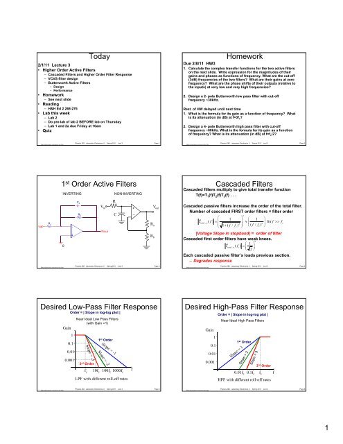
<strong>Today</strong><br />
2/1/11 Lecture 3<br />
• Higher <strong>Order</strong> <strong>Active</strong> <strong>Filters</strong><br />
– <strong>Cascaded</strong> <strong>Filters</strong> and Higher <strong>Order</strong> Filter Response<br />
– VCVS filter design<br />
– Butterworth <strong>Active</strong> <strong>Filters</strong><br />
• Design<br />
• Performance<br />
• <strong>Homework</strong><br />
– See next slide<br />
• Reading<br />
– H&H Ed 2 268-276<br />
• Lab this week<br />
– Lab 2<br />
– Do pre-lab of lab 2 BEFORE lab on Thursday<br />
– Lab 1 and 2a due Friday at 10am<br />
• Quiz<br />
<strong>Homework</strong><br />
Due 2/8/11 HW3<br />
1. Calculate the complex transfer functions for the two active filters<br />
on the next slide. Write expression for the magnitudes of their<br />
gains and phases as functions of frequency. What are the cut-off<br />
(3dB) frequencies of the two filters? What are their gains at zero<br />
frequency? What are the phase shifts of their outputs (relative to<br />
the inputs) at very low and very high frequencies?<br />
2. Design a 2- pole Butterworth low pass filter with cut-off<br />
frequency ~30kHz.<br />
Rest of HW delayed until next time<br />
1. What is the formula for its gain as a function of frequency? What<br />
is its attenuation (in dB) at f=3f c ?<br />
2. Design a 4- pole Butterworth high pass filter with cut-off<br />
frequency ~60kHz. What is the formula for its gain as a function<br />
of frequency? What is its attenuation (in dB) at f=f c /2?<br />
Based with permission on lectures by John Getty<br />
Physics 262: Laboratory Electronics II Spring 2011 Lect 3 Page 1<br />
Based with permission on lectures by John Getty<br />
Physics 262: Laboratory Electronics II Spring 2011 Lect 3 Page 2<br />
Vin<br />
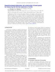
1 st <strong>Order</strong> <strong>Active</strong> <strong>Filters</strong><br />
INVERTING<br />
C 2<br />
R 1<br />
R 2<br />
0<br />
-<br />
+<br />
V in<br />
Vout<br />
R<br />
NON-INVERTING<br />
C<br />
+<br />
_<br />
R a<br />
R b<br />
V out<br />
<strong>Cascaded</strong> <strong>Filters</strong><br />
<strong>Cascaded</strong> filters multiply to give total transfer function<br />
T(f)=T 1 (f)T 2 (f)T 3 (f) . . .<br />
<strong>Cascaded</strong> passive filters increase the order of the total filter.<br />
Number of cascaded FIRST order filters = filter order<br />
1 1<br />
T<br />
<br />
( f) for f f<br />
<br />
<br />
<br />
( f / f )<br />
<br />
<br />
total _ n<br />
2<br />
n<br />
c<br />
1 ( f / fc<br />
) c <br />
|Voltage Slope in stopband| = order of filter<br />
<strong>Cascaded</strong> first order filters have weak knees.<br />
n<br />
1<br />
T<br />
<br />
total _ n( fc<br />
) <br />
2 <br />
Each cascaded passive filter’s loads previous section.<br />
– Degrades response<br />
n<br />
Based with permission on lectures by John Getty<br />
Physics 262: Laboratory Electronics II Spring 2011 Lect 3 Page 3<br />
Based with permission on lectures by John Getty<br />
Physics 262: Laboratory Electronics II Spring 2011 Lect 3 Page 4<br />
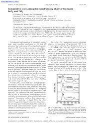
<strong>Desired</strong> Low-Pass Filter Response<br />
<strong>Order</strong> = | Slope in log-log plot |<br />
Near Ideal Low Pass <strong>Filters</strong><br />
(with Gain =1)<br />
Gain<br />
1<br />
1 st <strong>Order</strong><br />
0.1<br />
0.01<br />
0.001<br />
3 rd <strong>Order</strong><br />
f c 10f c 100f c 1000f c<br />
f<br />
LPF with different roll-off rates<br />
<strong>Desired</strong> High-Pass Filter Response<br />
<strong>Order</strong> = | Slope in log-log plot |<br />
Near Ideal High Pass <strong>Filters</strong><br />
Gain<br />
1<br />
1 st <strong>Order</strong><br />
0.1<br />
0.01<br />
0.001<br />
3 rd <strong>Order</strong><br />
0.01f c 0.1f c f c f<br />
HPF with different roll-off rates<br />
Based with permission on lectures by John Getty<br />
Physics 262: Laboratory Electronics II Spring 2011 Lect 3 Page 5<br />
Based with permission on lectures by John Getty<br />
Physics 262: Laboratory Electronics II Spring 2011 Lect 3 Page 6<br />
1
<strong>Cascaded</strong> <strong>Active</strong> <strong>Filters</strong><br />
<strong>Cascaded</strong> passive filters increase the order of the total filter.<br />
Same is true for active filters<br />
Each cascaded passive filter’s loads previous section.<br />
Not true with active filters<br />
• OpAmp has low current input => High input impedance<br />
• OpAmp provides lots of current => Low output impedance<br />
<strong>Cascaded</strong> first order filters have weak knees.<br />
True with active filters<br />
But . . .<br />
By crafting filter designs in cascaded active filters<br />
• Sharper knees, better time response, OR flatter phase response<br />
V in<br />
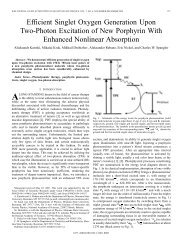
Sallen-Key 2 nd <strong>Order</strong> Low-Pass Filter<br />
A.K.A. Low Pass VCVS (voltage-controlled voltage-source)<br />
R 1 R 2<br />
+<br />
_<br />
C 2<br />
C 1<br />
V out<br />
Passband Gain = K<br />
Dual filtering at high f<br />
R a =(K-1)R b<br />
Different filter designs have<br />
R b -Different K values<br />
-Different RC values<br />
•RC determines f c , BUT<br />
•f c not always 1/(2RC)<br />
The roll-off rate for a two-pole (2 nd order) filter is<br />
20 decades/decade in Voltage OR -40 dB/decade in POWER.<br />
Based with permission on lectures by John Getty<br />
Physics 262: Laboratory Electronics II Spring 2011 Lect 3 Page 7<br />
Based with permission on lectures by John Getty<br />
Physics 262: Laboratory Electronics II Spring 2011 Lect 3 Page 8<br />
Design of 2 nd <strong>Order</strong> <strong>Active</strong> <strong>Filters</strong><br />
All the 2 nd order active filter circuits have the same basic design<br />
– Frequency selective RC circuit can be<br />
• Band-pass (see H&H Figure 5.16)<br />
• Low-pass<br />
R<br />
• High-pass<br />
C<br />
C<br />
R<br />
R<br />
C<br />
R<br />
C<br />
V in<br />
Frequency<br />
selective<br />
RC circuit<br />
Higher order (>2) active filters are cascaded 2 nd order circuits<br />
– Built up by cascading basic filter circuits: V out_previous => V in_next<br />
– Only one VCVS and one op-amp is needed per every two orders<br />
+<br />
_<br />
R a<br />
R b<br />
V out<br />
2 nd <strong>Order</strong> Butterworth Design<br />
1-stage (2-pole) filter design:<br />
Start with desire f c<br />
Butterworth: RC=1/(2f c ) and R a =(K-1)R b<br />
Typically R b =R in RC<br />
R is typically 10-100K ohm.<br />
(not hard rule)<br />
Butterworth Bessel<br />
Poles K f n K<br />
2 1.59 1.27 1.27<br />
V in<br />
Frequency<br />
selective<br />
RC circuit<br />
+<br />
_<br />
R a<br />
R b<br />
V out<br />
Based with permission on lectures by John Getty<br />
Physics 262: Laboratory Electronics II Spring 2011 Lect 3 Page 9<br />
Based with permission on lectures by John Getty<br />
Physics 262: Laboratory Electronics II Spring 2011 Lect 3 Page 10<br />
Higher <strong>Order</strong> Butterworth Design<br />
VCVS Low-Pass Filter Design:<br />
R<br />
C<br />
R<br />
f c is desired 3dB frequency<br />
of total n-pole filter<br />
C<br />
Butterworth Bessel<br />
Poles Stage(n) K n f n K n<br />
2 1 1.59 1.27 1.27<br />
4 1 1.15 1.43 1.08<br />
2 2.24 1.61 1.76<br />
6 1 1.07 1.61 1.04<br />
2 1.59 1.69 1.36<br />
3 2.48 1.91 2.02<br />
Butterworth:<br />
RC circuit is the same for all stages (Determined by desired f c )<br />
Only the gain changes for each stage<br />
RC=1/(2f c ) and R a =(K n -1)R b<br />
Typically gains increase down the line to avoid dynamic range issues<br />
Total Gain of multi-stage filter = product of the K n ’s<br />
For high pass filter: Same design table except:<br />
Use high pass VCVS<br />
Use 1/f n to determine RC<br />
2-stage (4-pole) Filter designs:<br />
Butterworth:<br />
R 1 C 1 = R 2 C 2 =1/(2f c )<br />
R a1 = (K 1 -1)R b1 = (1.15-1)R b1<br />
R a2 = (K 2 -1)R b1 = (2.24-1)R b2<br />
V in<br />
Frequency<br />
selective<br />
R 1 C 1 circuit<br />
4 th <strong>Order</strong> Butterworth<br />
Stage 1<br />
Frequency<br />
Stage 2<br />
+ V out V in selective +<br />
_<br />
R 2 C 2 circuit _<br />
R a1 =(K 1 -1)R b1<br />
R b1<br />
Butterworth Bessel<br />
Poles Stage(n) K n f n K n<br />
4 1 1.15 1.43 1.08<br />
2 2.24 1.61 1.76<br />
R 1 = R b1<br />
R 2 = R b2<br />
V out<br />
R a2 =(K 2 -1)R b2<br />
R b2<br />
Based with permission on lectures by John Getty<br />
Physics 262: Laboratory Electronics II Spring 2011 Lect 3 Page 11<br />
Based with permission on lectures by John Getty<br />
Physics 262: Laboratory Electronics II Spring 2011 Lect 3 Page 12<br />
2
Power<br />
Gain (dB)<br />
T<br />
( f)<br />
<br />
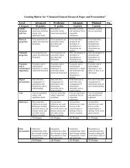
Butterworth Response<br />
1<br />
2<br />
(1 ( f / f ) n<br />
c<br />
T<br />
( f)<br />
<br />
1<br />
2<br />
Voltage<br />
Gain: T(f)<br />
1<br />
0.1<br />
0.01<br />
0.001<br />
0.0001<br />
0.00001<br />
0.000001<br />
Butterworth High Pass Filter Response<br />
Same design table except:<br />
Use high pass VCVS<br />
Use 1/f n to determine RC<br />
n=1<br />
2<br />
3<br />
4<br />
5<br />
6<br />
<strong>Order</strong> n<br />
T<br />
( f)<br />
<br />
T<br />
( f)<br />
<br />
1<br />
2<br />
1<br />
f<br />
2<br />
(1 ( / ) n<br />
c<br />
f<br />
Voltage<br />
Gain: T(f)<br />
1<br />
0.1<br />
0.01<br />
0.001<br />
0.0001<br />
0.00001<br />
0.000001<br />
f/f c<br />
Based with permission on lectures by John Getty<br />
Physics 262: Laboratory Electronics II Spring 2011 Lect 3 Page 13<br />
Based with permission on lectures by John Getty<br />
Physics 262: Laboratory Electronics II Spring 2011 Lect 3 Page 14<br />
R1<br />
10kohm<br />
V1<br />
1V<br />
0.71V_rms<br />
1000Hz<br />
0Deg<br />
Based with permission on lectures by John Getty<br />
Review Butterworth Design<br />
R2<br />
10kohm<br />
Swap the<br />
locations of<br />
the caps and<br />
resistors to<br />
change the<br />
type of filter.<br />
C1<br />
0.01uF<br />
C3<br />
0.01uF<br />
1<br />
2<br />
R3<br />
U1<br />
12.3kohm<br />
1.5kom<br />
R6<br />
10kohm<br />
Choose caps and<br />
resistors to adjust<br />
cut-off frequency. Use<br />
resistor in RC that is<br />
equal to or close to R b<br />
3<br />
R4<br />
10kohm<br />
Physics 262: Laboratory Electronics II Spring 2011 Lect 3 Page 15<br />
R5<br />
10kohm<br />
Same caps and<br />
resistors in each stage,<br />
sets cut-off frequency.<br />
Gains are set by<br />
the Butterworth<br />
polynomial and<br />
should not be<br />
changed<br />
C2<br />
0.01uF<br />
C4<br />
0.01uF<br />
1<br />
2<br />
R8<br />
10kohm<br />
U2<br />
Different gains in<br />
each stage, as per<br />
design table.<br />
R7<br />
3<br />
1.5kohm<br />
12.4kom<br />
3