Chapter 6

57:020 Mechanics of Fluids and Transport Processes Chapter 6 

Professor Fred Stern Fall 2013 

1 

Chapter 6 Differential Analysis of Fluid Flow 

Fluid Element Kinematics 

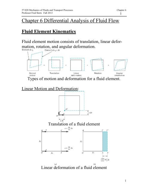
Fluid element motion consists of translation, linear deformation, 

rotation, and angular deformation. 

Types of motion and deformation for a fluid element. 

Linear Motion and Deformation: 

Translation of a fluid element 

Linear deformation of a fluid element 

1



2 

Change in: 

 

u 

x y z 

t 

x 

 

the rate at which the volume is changing per unit volume 

due to the gradient ∂u/∂x is 

1 

 

 

d u x t u 

lim 

dt t 

 

0 

t x 

If velocity gradients ∂v/∂y and ∂w/∂z are also present, then 

using a similar analysis it follows that, in the general case, 

 

 

1 d u v w 

V 

dt x y z 

This rate of change of the volume per unit volume is called 

the volumetric dilatation rate. 

Angular Motion and Deformation 

For simplicity we will consider motion in the x–y plane, 

but the results can be readily extended to the more general 

case. 

2



3 

Angular motion and deformation of a fluid element 

The angular velocity of line OA, ω OA , is 

 

OA 

lim 

t0 

t 

For small angles 

v xxt v tan t 

x x 

so that 

v x 

t v 

OA 

lim 

t0 

t 

x 

Note that if ∂v/∂x is positive, ω OA will be counterclockwise. 

Similarly, the angular velocity of the line OB is 

 

OB 

u 

lim 

t0 

t 

y 

In this instance if ∂u/∂y is positive, ω OB will be clockwise. 

3



4 

The rotation, ω z , of the element about the z axis is defined 

as the average of the angular velocities ω OA and ω OB of the 

two mutually perpendicular lines OA and OB. Thus, if 

counterclockwise rotation is considered to be positive, it 

follows that 

1 v 

u 

z 

 

2 x 

y 

Rotation of the field element about the other two coordinate 

axes can be obtained in a similar manner: 

1 w 

v 

x 

 

2 y 

z 

1 u 

w 

 

y 

 

2 z 

x 

 

The three components, ω x ,ω y , and ω z can be combined to 

give the rotation vector, ω, in the form: 

1 1 

ω xi yj zk curlV V 

2 2 

since 

i j k 

1 1 

V 

2 2 x y z 

u v w 

1 w v 1 u w 1 v u 

 

i j k 

2 y z 2 z x 2 x y 

 

4

̇ 

̇ 



5 

The vorticity, ζ, is defined as a vector that is twice the rotation 

vector; that is, 

2ω V 

The use of the vorticity to describe the rotational characteristics 

of the fluid simply eliminates the (1/2) factor associated 

with the rotation vector. If V 0 , the flow is 

called irrotational. 

In addition to the rotation associated with the derivatives 

∂u/∂y and ∂v/∂x, these derivatives can cause the fluid element 

to undergo an angular deformation, which results in a 

change in shape of the element. The change in the original 

right angle formed by the lines OA and OB is termed the 

shearing strain, δγ, 

 

The rate of change of δγ is called the rate of shearing strain 

or the rate of angular deformation: 

̇ [ ( ⁄ ) ( ⁄ ) ] 

Similarly, 

The rate of angular deformation is related to a corresponding 

shearing stress which causes the fluid element to 

change in shape. 

5



6 

The Continuity Equation in Differential Form 

The governing equations can be expressed in both integral 

and differential form. Integral form is useful for large-scale 

control volume analysis, whereas the differential form is 

useful for relatively small-scale point analysis. 

Application of RTT to a fixed elemental control volume 

yields the differential form of the governing equations. For 

example for conservation of mass 

V 

A 

CS 

 

 

CV 

 

dV 

t 

net outflow of mass = rate of decrease 

across CS 

of mass within CV 

6



7 

Consider a cubical element oriented so that its sides are to 

the (x,y,z) axes 

 

 

u 

x 

 

 

outlet mass flux 

u 

dx 

dydz 

inlet mass flux 

udydz 

Taylor series expansion 

retaining only first order term 

We assume that the element is infinitesimally small such 

that we can assume that the flow is approximately one dimensional 

through each face. 

The mass flux terms occur on all six faces, three inlets, and 

three outlets. Consider the mass flux on the x faces 

x 

 

 

 

ρu ρudx dydz 

x 

 

 

ρudydz 

 

= ( u) dxdydz 

x 

V 

flux outflux influx 

Similarly for the y and z faces 

 

yflux 

( v)dxdydz 

y 

z 

flux 

 

( w)dxdydz 

z 

7



8 

The total net mass outflux must balance the rate of decrease 

of mass within the CV which is 

 

dxdydz 

t 

Combining the above expressions yields the desired result 

 

 

( u) 

( v) 

( w) 

dxdydz 0 

t x y z 

 

 

dV 

 

 

t 

 

 

( u) 

 

x 

 

( v) 

 

y 

 

 

( w) 

z 

0 

per unit V 

differential form of continuity 

equations 

 

( 

V) 

0 

t 

 

V V 

D 

V 

Dt 

0 

D 

Dt 

 

 

t 

V 

Nonlinear 1 st order PDE; ( unless = constant, then linear) 

Relates V to satisfy kinematic condition of mass conservation 

Simplifications: 

1. Steady flow: ( V) 

0 

2. = constant: V 0 

8



9 

u 

v 

w 

i.e., 0 

x 

y 

z 

3D 

u 

x 

 

v 

y 

0 

2D 

The continuity equation in Cylindrical Polar Coordinates 

The velocity at some arbitrary point P can be expressed as 

V vrer ve 

vze 

z 

The continuity equation: 

 

1rvr 1v 

v 

 

z 

0 

t r r r 

z 

For steady, compressible flow 

1rvr 1v 

vz 

0 

r r r 

z 

For incompressible fluids (for steady or unsteady flow) 

1rvr 

1v 

vz 

0 

r r r 

z 

9



10 

The Stream Function 

Steady, incompressible, plane, two-dimensional flow represents 

one of the simplest types of flow of practical importance. 

By plane, two-dimensional flow we mean that 

there are only two velocity components, such as u and v, 

when the flow is considered to be in the x–y plane. For this 

flow the continuity equation reduces to 

u 

v 

0 

x 

y 

We still have two variables, u and v, to deal with, but they 

must be related in a special way as indicated. This equation 

suggests that if we define a function ψ(x, y), called the 

stream function, which relates the velocities as 

 

 

u , v 

y 

x 

then the continuity equation is identically satisfied: 

2 2 

 

0 

x y y x xy xy 

Velocity and velocity components along a streamline 

10



11 

Another particular advantage of using the stream function 

is related to the fact that lines along which ψ is constant are 

streamlines.The change in the value of ψ as we move from 

one point (x, y) to a nearby point (x + dx, y + dy) along a 

line of constant ψ is given by the relationship: 

 

d dx dy vdx udy 0 

x 

y 

and, therefore, along a line of constant ψ 

dy v 

 

dx u 

The flow between two streamlines 

The actual numerical value associated with a particular 

streamline is not of particular significance, but the change 

in the value of ψ is related to the volume rate of flow. Let 

dq represent the volume rate of flow (per unit width perpendicular 

to the x–y plane) passing between the two 

streamlines. 

 

 

dq udy vdx dx dy d 

x 

y 

Thus, the volume rate of flow, q, between two streamlines 

such as ψ1 and ψ2, can be determined by integrating to 

yield: 

11



12 

q 

 

 

2 

d 

1 

 

2 1 

In cylindrical coordinates the continuity equation for incompressible, 

plane, two-dimensional flow reduces to 

1rvr 

1v 

0 

r r r 

and the velocity components, v r and v θ , can be related to the 

stream function, ψ(r, θ), through the equations 

1 

 

vr 

, v 

 

r 

r 

Navier-Stokes Equations 

Differential form of momentum equation can be derived by 

applying control volume form to elemental control volume 

The differential equation of linear momentum: elemental 

fluid volume approach 

12



13 

⏟ 

∫ 

( ) 

∫ 

⏟ 

( ) 

̂ 

(1) = ( ) ( ) 

(2) = [ ( ) ⏟ ( ) 

⏟ 

⏟ ( )] 

=[ ] 

combining and making use of the continuity equation yields 

[ { ( ) 

⏟ } ( )] 

or 

where 

13



14 

Body forces are due to external fields such as gravity or 

magnetics. Here we only consider a gravitational field; that 

is, 

F 

and 

i.e., 

dFgrav 

gdxdydz 

g gkˆ 

for g z 

f body gkˆ 

body 

Surface forces are due to the stresses that act on the sides of 

the control surfaces 

symmetric ( ij = ji ) 

ij = - p ij + ij 

2 nd order tensor 

normal pressure 

viscous stress 

ij = 1 

ij = 0 

i = j 

i j 

= -p+ xx xy xz 

yx -p+ yy yz 

zx zy -p+ zz 

As shown before for p alone it is not the stresses themselves 

that cause a net force but their gradients. 

 

 

x 

 

y 

 

z 

dF x,surf = 

 

 

 

 

dxdydz 

 

 

 

p 

x 

xx 

 

x 

xy 

 

y 

= 

 

 

 

 

dxdydz 

xx 

xy 

xz 

 

 

 

z 

xz 

 

 

14



15 

This can be put in a more compact form by defining vector 

stress on x-face 

 

x 

 

xx 

î 

xy 

ĵ 

 

xz 

kˆ 

and noting that 

p 

 

dF x,surf = 

 

x dxdydz 

x 

 

p 

f x,surf = x 

per unit volume 

x 

similarly for y and z 

p 

f y,surf = y 

y yxî 

yyĵ 

yzkˆ 

y 

f z,surf = 

p 

z 

z zxî 

zyĵ 

zzkˆ 

z 

finally if we define 

î ĵ 

kˆ then 

ij 

x 

y 

z 

f 

surf 

p 

ij 

ij 

ij pij 

ij 

15



16 

Putting together the above results 

f 

f 

body 

f 

surf 

 

DV 

Dt 

f body gkˆ 

f p 

 

surface 

DV V 

a VV 

Dt t 

ij 

a gkˆ 

p 

 

ij 

inertia body 

force force surface surface force 

due to force due due to viscous 

gravity to p shear and normal 

stresses 

16



17 

For Newtonian fluid the shear stress is proportional to the 

rate of strain, which for incompressible flow can be written 

( ) 

where, 

= coefficient of viscosity 

= rate of strain tensor 

( ) ( ) 

= 

( ) ( ) 

[ 

( ) ( ) 

] 

Ex) 1-D flow 

̂ ( ) 

where, 

( ) ( ) 

⏟ ⏟ 

( 

) 

̂ 

( ) Navier-Stokes Equation 

Continuity Equation 

17



18 

Four equations in four unknowns: V and p 

Difficult to solve since 2 nd order nonlinear PDE 

x: [ ] [ ] 

y: [ ] [ ] 

z: [ ] [ ] 

u 

x 

v 

 

y 

w 

 

z 

0 

Navier-Stokes equations can also be written in other coordinate 

systems such as cylindrical, spherical, etc. 

There are about 80 exact solutions for simple geometries. 

For practical geometries, the equations are reduced to algebraic 

form using finite differences and solved using computers. 

18



19 

Ex) Exact solution for laminar incompressible steady flow 

in a circular pipe 

Use cylindrical coordinates with assumptions 

: Fully-developed flow 

: Flow is parallel to the wall 

Continuity equation: 

( ) 

i.e., 

B.C. ( ) 

19



20 

Momentum equation: 

( ) 

[ ( ) ] 

( ) 

[ ( ) ] 

( ) 

[ ( ) ] 

or 

(1) 

(2) 

[ ( )] (3) 

where, 

Equations (1) and (2) can be integrated to give 

( ) ( ) ( ) 

pressure is hydrostatic and ⁄ is not a function 

of or 

20



21 

Equation (3) can be written in the from 

( ) 

and integrated (using the fact that ⁄ = constant) to 

give 

( ) 

Integrating again we obtain 

( ) 

B.C. 

( ) 

( ) ( ) 

( ) ( ) 

at any cross section the velocity distribution is parabolic 

21



22 

1) Flow rate : 

∫ ∫ ( ) 

where, ( ) 

If the pressure drops over a length : 

2) Mean velocity : 

( ) ( ) 

3) Maximum velocity : 

( ) ( ) 

 

( ) 

22



23 

4) Wall shear stress ( ) : 

( ) 

where 

⏟ ( ) 

Thus, at the wall (i.e., ), 

( ) 

and with , 

|( ) | 

Note: Only valid for laminar flows. In general, the flow 

remains laminar for Reynolds numbers, Re = ( ) ⁄ , 

below 2100. Turbulent flow in tubes is considered in Chapter 

8. 

23



24 

Differential Analysis of Fluid Flow 

We now discuss a couple of exact solutions to the Navier- 

Stokes equations. Although all known exact solutions 

(about 80) are for highly simplified geometries and flow 

conditions, they are very valuable as an aid to our understanding 

of the character of the NS equations and their solutions. 

Actually the examples to be discussed are for internal 

flow (Chapter 8) and open channel flow (Chapter 

10), but they serve to underscore and display viscous flow. 

Finally, the derivations to follow utilize differential analysis. 

See the text for derivations using CV analysis. 

Couette Flow 

boundary conditions 

First, consider flow due to the relative motion of two parallel 

plates 

u Continuity 0 

x 

d u 

Momentum 0 

2 

dy 

2 

u = u(y) 

v = o 

p 

p 

 

x 

y 

0 

or by CV continuity and momentum equations: 

24



25 

u y 

u 

2 

u 1 = u 2 

1 

y 

 

Fx 

uV 

dA 

Q u2 

u1 

0 

dp d 

 

py 

p 

xy 

x 

dyx 

= 0 

dx dy 

d 

0 

dy 

d du 

i.e. 0 

dy dy 

2 

d u 

0 

2 

dy 

from momentum equation 

 

du C 

dy 

C 

u y 

 

D 

u(0) = 0 D = 0 

U 

u y 

t 

du 

 

dy 

u(t) = U C = 

U 

 

t 

U 

 

t 

constant 

25



26 

Generalization for inclined flow with a constant pressure 

gradient 

u Continutity 0 

x 

d u 

0 p z 

 

x 

dy 

Momentum 

2 

2 

u = u(y) 

v = o 

p 

0 

y 

i.e., 

2 

d u dh 

h = p/ +z = constant 

2 

dy dx 

which can be integrated twice to yield 

 

du 

dy 

u 

 

dh 

dx 

dh 

dx 

y 

2 

y A 

2 

Ay B 

dz 

plates horizontal 0 

dx 

dz 

plates vertical =-1 dx 

26



27 

now apply boundary conditions to determine A and B 

u(y = 0) = 0 B = 0 

u(y = t) = U 

U 

 

dh 

dx 

2 

t 

2 

At 

A 

 

U 

t 

 

dh 

dx 

t 

2 

dh y 

u(y) 

dx 2 

dh 

 

2 

dx 

2 

1 U 

 

 

 

t 

U 

ty y 

2 

t 

dh 

dx 

= y 

This equation can be put in non-dimensional form: 

2 

u t 

dh y y y 

1 

 

U 2U 

dx t t t 

t 

2 

 

 

 

define: P = non-dimensional pressure gradient 

t 2 dh 

p 

= h z 

2U 

dx 

 

Y = y/t 

u 

PY(1 

Y) Y 

U 

parabolic velocity profile 

1 dp 

 

2U 

 

 

dx 

z 2 

 

dz 

dx 

 

 

27



28 

u 

U 

 

2 

Py Py 

 

2 

t t 

 

y 

t 

q 

u 

t 

udy 

 

0 

q 

t 

t 

 

U 

0 

 

t 

 

dy 

tu 

U 

t 0 

P 

 

y 

t 

P 2 y 

y 

2 

dy 

t t 

= 

Pt 

2 

 

Pt 

3 

 

t 

2 

u 

U 

 

P 

6 

 

1 

2 

u 

2 

t 

 

12 

 

dh 

 

dx 

U 

2 

ut 

For laminar flow 1000 

 

Re crit 1000 

28



29 

The maximum velocity occurs at the value of y for which: 

du d u P 2P 1 

0 0 y 

2 

dy dy U t t t 

t t t 

y P 

1 

@ u max 

2P 2 2P 

for U = 0, y = t/2 

 

u 

max 

u 

 

y 

max 

 

 

UP 

4 

 

U 

2 

 

U 

4P 

note: if U = 0: 

u 

u 

max 

 

P 

6 

P 

4 

 

2 

3 

The shape of the velocity profile u(y) depends on P: 

dh 

1. If P > 0, i.e., 0 the pressure decreases in the 

dx 

direction of flow (favorable pressure gradient) and the 

velocity is positive over the entire width 

 

dh 

dx 

 

d 

dx 

 

 

 

p 

 

 

z 

 

 

dp 

dx 

sin 

 

dp 

a) 0 

dx 

dp 

b) sin 

 

dx 

29



30 

1. If P < 0, i.e., dh dx 0 the pressure increases in the direction 

of flow (adverse pressure gradient) and the velocity 

over a portion of the width can become negative 

(backflow) near the stationary wall. In this case the 

dragging action of the faster layers exerted on the fluid 

particles near the stationary wall is insufficient to overcome 

the influence of the adverse pressure gradient. 

dp 

dx 

dp 

sin 

0 

sin 

 

dx 

or 

sin 

dp 

dx 

dh 

2. If P = 0, i.e., 0 the velocity profile is linear 

dx 

U 

u y 

t 

dp 

a) 0 and = 0 Note: we derived 

dx 

this special case 

dp 

b) sin 

 

dx 

u 

For U = 0 the form PY1 

Y 

Y is not appropriate 

U 

u = UPY(1-Y)+UY 

t 2 dh 

= Y1 

Y 

UY 

2 

dx 

t 

2 

dh 

dx 

Now let U = 0: u Y1 

Y 

2 

30



31 

3. Shear stress distribution 

Non-dimensional velocity distribution 

where 

u 

U 

2 

t dh 

P 

2U dx 

y 

Y 

t 

* u 

Shear stress 

u 

U 

* 

u PY 1Y Y 

is the non-dimensional velocity, 

 

 

is the non-dimensional pressure gradient 

is the non-dimensional coordinate. 

du 

 

dy 

In order to see the effect of pressure gradient on shear 

stress using the non-dimensional velocity distribution, we 

define the non-dimensional shear stress: 

Then 

where 

* 

 

* 

 

 

1 

 

2 U 

2 

 

 

 

 

1 Ud u U 2 

du 

 

1 2 

U 

td y t Ut dY 

2 

2 

2PY 

P 1 

Ut 

2 

2PY 

P 1 

Ut 

 

A 2PY P 1 

2 

A 0 is a positive constant. 

Ut 

So the shear stress always varies linearly with Y across any 

section. 

 

* 

31



32 

At the lower wall Y 0 

: 

At the upper wall 

 

* 

1 

lw 

A P 

1 

 

* 

1 

 

Y : 

uw 

A P 

For favorable pressure gradient, the lower wall shear stress 

is always positive: 

1. For small favorable pressure gradient 0P 

1 

: 

* 

0 and 0 

* 

lw 

2. For large favorable pressure gradient 1 

* 

lw 

uw 

0 and 0 

* 

uw 

P : 

 

 

 

P 

 

P 1 

0 1 

For adverse pressure gradient, the upper wall shear stress is 

always positive: 

1. For small adverse pressure gradient 1 P 0: 

* 

0 and 0 

* 

lw 

2. For large adverse pressure gradient 1 

* 

lw 

uw 

* 

0 and 0 

uw 

P : 

32



33 

 

 

1 P 0 

P 1 

For U 0 , i.e., channel flow, the above non-dimensional 

form of velocity profile is not appropriate. Let’s use dimensional 

form: 

2 

t dh 

dh 

u 

 

Y Y y t y 

2 

dx 

2 

dx 

 

1 

 

Thus the fluid always flows in the direction of decreasing 

piezometric pressure or piezometric head because 

 

0, y 0 

2 and ty 0 . So if dh 

dx is negative, u is positive; 

if dh 

dx is positive, u is negative. 

Shear stress: 

du dh 1 

t y 

dy 2 dx 2 

Since 

1 

t 

y0 

2 

, the sign of shear stress is always opposite 

to the sign of piezometric pressure gradient dh 

, and the 

magnitude of is always maximum at both walls and zero 

at centerline of the channel. 

dx 

33



34 

dh 

For favorable pressure gradient, 0 

dx , 0 

For adverse pressure gradient, 0 

dx , 0 

dh 

Flow down an inclined plane 

dh 

0 

dx dh 

0 

dx 

uniform flow velocity and depth do not 

change in x-direction 

Continuity 0 

dx 

 

du 

 

34



35 

d u 

x-momentum 0 p 

z 

 

2 

x 

dy 

 

y-momentum p 

z 

y 

dp 0 

dx 

0 hydrostatic pressure variation 

2 

2 

d u 

 

2 

dy 

sin 

 

du 

dy 

 

 

 

sin y 

c 

u 

2 

y 

sin 

2 

Cy D 

du 

dy 

yd 

0 

 

 

 

sin d 

c c 

 

 

 

sin d 

u(0) = 0 D = 0 

u 

2 

y 

sin 

2 

 

 

sin dy 

 

 

2 

= sin y2d 

y 

35



36 

gsin 

2 

u(y) = y2d 

y 

q 

 

d 

3 

 

2 y 

udy sin dy 

 

0 2 

3 

= 1 

d 

3 sin 

3 

 

 

 

 

 

d 

0 

discharge per 

unit width 

V 

avg 

 

q 

d 

 

1 

3 

 

 

d 

2 

sin 

2 

gd 

3 

sin 

in terms of the slope S o = tan sin 

V 

 

2 

gd S 

3 

o 

Exp. show Re crit 500, i.e., for Re > 500 the flow will become 

turbulent 

p 

y 

cos 

Re 

Vd 

crit 500 

 

p cos 

y C 

d 

p po cosd 

C 

36



37 

p cos 

d y 

p 

i.e., o 

* p(d) > p o 

* if = 0 p = (d y) + p o 

entire weight of fluid imposed 

if = /2 

p = p o 

no pressure change through the fluid 

37

Chapter 6

You also want an ePaper? Increase the reach of your titles

Delete template?

Save as template?