November 2001 - Course 1 SOA Solutions
November 2001 - Course 1 SOA Solutions
November 2001 - Course 1 SOA Solutions

You also want an ePaper? Increase the reach of your titles
YUMPU automatically turns print PDFs into web optimized ePapers that Google loves.
<strong>Course</strong> 1 <strong>Solutions</strong><br />
<strong>November</strong> <strong>2001</strong> Exams
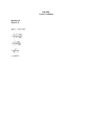
1. A<br />
For i = 1, 2, let<br />
R = event that a red ball is drawn form urn i<br />
i<br />
B = event that a blue ball is drawn from urn i .<br />
i<br />
Then if x is the number of blue balls in urn 2,<br />
( R1∩R2) ∪( B1∩B2) R1∩R2 [ B1∩B2]<br />
[ R ] [ R ] + [ B ] [ B ]<br />
0.44 = Pr[ ] = Pr[ ] + Pr<br />
= Pr Pr Pr Pr<br />
1 2 1 2<br />
4 ⎛ 16 ⎞ 6 ⎛ x ⎞<br />
= ⎜ ⎟+<br />
⎜ ⎟<br />
10 ⎝ x+ 16 ⎠ 10 ⎝ x+<br />
16 ⎠<br />
Therefore,<br />
32 3x<br />
3x+<br />
32<br />
2.2 = + =<br />
x+ 16 x+ 16 x+<br />
16<br />
2.2x+ 35.2 = 3x+<br />
32<br />
0.8x<br />
= 3.2<br />
x = 4<br />
2. C<br />
We are given that<br />
f x, y dA= 6 and dA=<br />
2<br />
∫∫ R<br />
( )<br />
∫∫ R<br />
It follows that<br />
∫∫⎡4 ( , ) 2 4 ( , ) 2<br />
R ⎣ f xy− ⎤⎦dA= ∫∫f xydA−<br />
dA<br />
R ∫∫ R<br />
= 4 6 − 2 2 = 20<br />
( ) ( )<br />
<strong>Course</strong> 1 <strong>Solutions</strong> 1 <strong>November</strong> <strong>2001</strong>
3. A<br />
Since<br />
3 4 2 5<br />
S = 175L A , we have<br />
∂ S<br />
1 4<br />
=<br />
2 5<br />
262.5 L A > 0 for<br />
∂L<br />
L > 0 , A > 0<br />
2<br />
∂ S<br />
− 1 4<br />
2 5<br />
= 131.25 L A > 0 for<br />
2<br />
∂L<br />
L> 0 , A><br />
0<br />
∂ S<br />
3 −1 = 140 L 2<br />
A 5 > 0 for<br />
∂A<br />
L > 0 , A > 0<br />
2<br />
∂ S<br />
3 −6<br />
2 5<br />
=− 28 L A < 0 for<br />
2<br />
∂A<br />
L> 0 , A><br />
0<br />
It follows that S increases at an increasing rate as L increases, while S increases at a<br />
decreasing rate as A increases.<br />
4. B<br />
Apply Baye’s Formula:<br />
Pr ⎡⎣Seri. Surv. ⎤⎦<br />
=<br />
Pr ⎡⎣Surv. Seri. ⎤⎦Pr[ Seri. ]<br />
Pr ⎡⎣Surv. Crit. ⎤ ⎦Pr[ Crit. ] + Pr ⎡⎣Surv. Seri. ⎤ ⎦Pr[ Seri. ] + Pr ⎡⎣Surv. Stab. ⎤⎦Pr[ Stab. ]<br />
( 0.9)( 0.3)<br />
0.29<br />
( 0.6)( 0.1) + ( 0.9)( 0.3) + ( 0.99)( 0.6)<br />
= =<br />
<strong>Course</strong> 1 <strong>Solutions</strong> 2 <strong>November</strong> <strong>2001</strong>
5. A<br />
Let us first determine K. Observe that<br />
⎛ 1 1 1 1 ⎞ ⎛60 + 30 + 20 + 15 + 12 ⎞ ⎛137<br />
⎞<br />
1= K⎜1+ + + + ⎟= K⎜ ⎟=<br />
K⎜ ⎟<br />
⎝ 2 3 4 5 ⎠ ⎝ 60 ⎠ ⎝ 60 ⎠<br />
60<br />
K =<br />
137<br />
It then follows that<br />
Pr N = n = Pr ⎣⎡ N = n Insured Suffers a Loss⎤⎦Pr Insured Suffers a Loss<br />
60 3<br />
= ( 0.05 ) = , N = 1,...,5<br />
137N<br />
137N<br />
P = E X where<br />
[ ] [ ]<br />
Now because of the deductible of 2, the net annual premium [ ]<br />
⎧0 , if N ≤ 2<br />
X = ⎨<br />
⎩N<br />
− 2 , if N > 2<br />
Then,<br />
P E [ X 5<br />
] ( N 3 ⎛ 1 ⎞ ⎡ 3 ⎤ ⎡ 3 ⎤<br />
= = ∑ − 2) = () 1 2 3 0.0314<br />
N = 3<br />
⎜ ⎟+ ⎢ ⎥+ ⎢ ⎥ =<br />
137N<br />
⎝137 ⎠ ⎣137( 4) ⎦ ⎣137( 5)<br />
⎦<br />
6. E<br />
The line 5y− 4x= 3 has slope 4 5<br />
4 dy dy dx 2t<br />
= = =<br />
5 dx dt dt 2t<br />
+ 1<br />
8t+ 4=<br />
10t<br />
2t<br />
= 4<br />
t = 2<br />
. It follows that we need to find t such that<br />
<strong>Course</strong> 1 <strong>Solutions</strong> 3 <strong>November</strong> <strong>2001</strong>
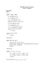
7. A<br />
Cov C , C = Cov X + Y, X + 1.2Y<br />
( 1 2) ( )<br />
= Cov ( X, X) + Cov ( Y, X) + Cov ( X,1.2Y) + Cov( Y,1.2Y)<br />
= Var X + Cov ( X, Y) + 1.2Cov ( X, Y)<br />
+ 1.2VarY<br />
= Var X + 2.2Cov ( X, Y)<br />
+ 1.2VarY<br />
( ) ( ( ))<br />
2<br />
( ) ( E Y )<br />
2 2<br />
2<br />
Var X = E X − E X = 27.4 − 5 = 2.4<br />
VarY<br />
2 2<br />
= E Y − ( ) = 51.4 − 7 = 2.4<br />
( X + Y) = X + Y + ( X Y)<br />
Var Var Var 2Cov ,<br />
1<br />
Cov ( XY , ) = Var ( X+ Y)<br />
−Var X−VarY<br />
2<br />
1<br />
= ( 8 − 2.4 − 2.4 ) = 1.6<br />
2<br />
Cov , = 2.4 + 2.2 1.6 + 1.2 2.4 = 8.8<br />
( C C ) ( ) ( )<br />
1 2<br />
( )<br />
<strong>Course</strong> 1 <strong>Solutions</strong> 4 <strong>November</strong> <strong>2001</strong>
7. Alternate solution:<br />
We are given the following information:<br />
C1<br />
= X + Y<br />
C2<br />
= X + 1.2Y<br />
E X = 5<br />
[ ]<br />
2<br />
⎡ ⎤ =<br />
E⎣X<br />
⎦<br />
EY = 7<br />
[ ]<br />
2<br />
⎡ ⎤ =<br />
27.4<br />
E⎣Y<br />
⎦ 51.4<br />
Var[ X + Y]<br />
= 8<br />
Now we want to calculate<br />
Cov C , C = Cov X + Y, X + 1.2Y<br />
( 1 2) ( )<br />
= E⎡⎣( X + Y)( X + 1.2Y) ⎤⎦− E[ X + Y] iE[ X + 1.2Y]<br />
2 2<br />
= ⎡<br />
⎣ + + ⎤<br />
⎦− [ ] + [ ] +<br />
2 2<br />
= E⎡ ⎣X ⎤<br />
⎦+ 2.2E[ XY] + 1.2E⎡ ⎣Y<br />
⎤<br />
⎦− ( 5 + 7) 5 + ( 1.2)<br />
7<br />
= 27. 4 + 2.2E[ XY] + 1.2( 51.4) −( 12)( 13.4)<br />
= 2.2E[ XY]<br />
−71.72<br />
Therefore, we need to calculate E [ XY ] first. To this end, observe<br />
2<br />
2<br />
8= Var[ X + Y] = E⎡( X + Y) ⎤− ( E[ X + Y]<br />
)<br />
[ ]<br />
E XY<br />
( )( [ ] [ ])<br />
( )<br />
E X 2.2XY 1.2Y E X E Y E X 1.2E Y<br />
⎣<br />
⎦<br />
2 2<br />
2<br />
= E ⎡<br />
⎣X + 2XY + Y ⎤<br />
⎦− ( E[ X] + E[ Y]<br />
)<br />
2 2<br />
2<br />
= E⎡ ⎣X ⎤<br />
⎦+ 2E[ XY] + E⎡ ⎣Y<br />
⎤<br />
⎦− ( 5 + 7)<br />
= 27.4 + 2E[ XY]<br />
+ 51.4 −144<br />
= 2E[ XY]<br />
−65.2<br />
( 8 65.2)<br />
2 36.6<br />
= + =<br />
Finally,<br />
Cov CC = 2.2 36.6 − 71.72 = 8.8<br />
( 1, 2 ) ( )<br />
<strong>Course</strong> 1 <strong>Solutions</strong> 5 <strong>November</strong> <strong>2001</strong>
8. D<br />
The function F() t , 1≤t<br />
≤ 7 , achieves its minimum value at one of the endpoints of the<br />
interval 1≤t<br />
≤ 7 or at t such that<br />
−t −t −t<br />
0= F′<br />
() t = e − te = e ( 1−t)<br />
Since F′ () t < 0 for t > 1 , we see that F () t is a decreasing function on the interval<br />
1< t ≤ 7 . We conclude that<br />
F 7 = 7e − = 0.0064<br />
( )<br />
7<br />
is the minimum value of F.<br />
9. D<br />
Let<br />
C = event that patient visits a chiropractor<br />
T = event that patient visits a physical therapist<br />
We are given that<br />
Pr[ C] = Pr[ T]<br />
+ 0.14<br />
Pr C∩T<br />
= 0.22<br />
( )<br />
c c<br />
( C ∩T<br />
)<br />
Pr = 0.12<br />
Therefore,<br />
c c<br />
0.88 = 1− Pr ⎡<br />
⎣C ∩T ⎤<br />
⎦ = Pr C∪T = Pr C + Pr T −Pr<br />
C∩T<br />
= Pr[ T] + 0.14 + Pr[ T]<br />
−0.22<br />
= 2 Pr T −0.08<br />
or<br />
[ ]<br />
Pr[ T ] = ( 0.88 + 0.08)<br />
2 = 0.48<br />
[ ] [ ] [ ] [ ]<br />
<strong>Course</strong> 1 <strong>Solutions</strong> 6 <strong>November</strong> <strong>2001</strong>
10. E<br />
Note that the terms of ∑ ∞ ⎛ 1 ⎞<br />
a<br />
n=<br />
1⎜<br />
n<br />
+ ⎟<br />
⎝ n ⎠<br />
exceed the terms of the harmonic series for<br />
1 1<br />
a = n<br />
1 , a = n<br />
, or an<br />
2<br />
n<br />
= n<br />
and will thus fail to converge.<br />
Moreover, the terms of the series<br />
n<br />
∞<br />
⎡( −1)<br />
1⎤<br />
∞ ⎛ 1 1 ⎞ ∞ 1<br />
∑ ⎢ + ⎥ =<br />
n= 1 ∑n= 1⎜ + ⎟=<br />
∑n=<br />
1<br />
⎢⎣<br />
n n⎥<br />
⎦ ⎝2n 2n⎠<br />
n<br />
are seen to be identical to the terms of the divergent harmonic series. By contrast, the<br />
series<br />
∞ ⎡ 1⎤ ∞ ⎡1−<br />
n 1⎤<br />
∞ 1<br />
∑ a<br />
n= 1⎢ n<br />
+<br />
n= 1 2 n=<br />
1 2<br />
n⎥ = ∑ + =<br />
⎣ ⎦<br />
⎢<br />
⎣ n n⎥<br />
∑<br />
⎦ n<br />
is seen to converge by the integral test, since<br />
∞<br />
2 1<br />
x −<br />
dx ∞<br />
∫ =−<br />
1 = 1
12. E<br />
Observe that<br />
x<br />
f′ x = f′′<br />
t dt<br />
For [ ]<br />
( ) ( )<br />
∫<br />
0<br />
= (area bounded by f′′<br />
above the x-axis from 0 to x)<br />
− (area bounded by f ′′ below the x-axis from 0 to x)<br />
x ∈ 0,5 , f ′′ is drawn such that the area bounded by f ′′ above the x-axis from 0 to<br />
x is strictly greater than the area bounded by f ′′ below the x-axis from 0 to x. Therefore,<br />
f′ ( x) > 0 for 0 < x≤ 5 . We conclude that f is an increasing function on the interval<br />
[ 0,5 ], and its maximum value occurs at x = 5 .<br />
13. E<br />
10 8<br />
F y Y y X y ⎡ X ⎤ e −<br />
⎣ ⎦ ⎢ 10 ⎥<br />
⎣<br />
⎦<br />
( )<br />
( ) [ ] ( ) 10 8<br />
0.8 10<br />
= Pr ≤ = Pr ⎡10 ≤ ⎤ = Pr ≤ Y = 1−<br />
Therefore, ( ) ′( )<br />
1 4<br />
10<br />
1 Y<br />
f y = F y = ⎛ ⎞<br />
⎜ ⎟ e −<br />
8⎝10⎠<br />
( Y ) 54<br />
Y<br />
14. A<br />
L’Hôspital’s Rule may be applied since f and g are given differentiable and from the<br />
diagram lim f( x) = lim g( x) = 0 .<br />
x→0 x→0<br />
f ( x)<br />
f′<br />
( x)<br />
Therefore lim = lim<br />
x→0 g ( x)<br />
x→0<br />
g′<br />
( x)<br />
Also from the diagram f′ ( x) f′<br />
( )<br />
This leads to<br />
lim = 0 > 0<br />
x→0<br />
and g′ ( x) x→0<br />
g′<br />
( )<br />
f ( x)<br />
f′ ( x)<br />
f′<br />
( 0)<br />
→0 g( x)<br />
x→0<br />
g′ ( x)<br />
g′<br />
( 0)<br />
lim = 0 < 0<br />
lim = lim = < 0<br />
x<br />
<strong>Course</strong> 1 <strong>Solutions</strong> 8 <strong>November</strong> <strong>2001</strong>
15. E<br />
Let X1,...,<br />
X<br />
100<br />
denote the number of pensions that will be provided to each new recruit.<br />
Now under the assumptions given,<br />
⎧0 with probability 1− 0.4 = 0.6<br />
⎪<br />
X i = ⎨1 with probability ( 0.4)( 0.25)<br />
= 0.1<br />
⎪<br />
⎩2 with probability ( 0.4)( 0.75)<br />
= 0.3<br />
for i = 1,...,100 . Therefore,<br />
E X = 0 0.6 + 1 0.1 + 2 0.3 = 0.7 ,<br />
[ i ] ( )( ) ( )( ) ( )( )<br />
2 2 2 2<br />
⎣ i ⎦ ( ) ( ) ( ) ( ) ( ) ( )<br />
2<br />
[ Xi] E⎡X ⎤<br />
i { E[ Xi]<br />
} ( )<br />
E⎡X<br />
⎤ = 0 0.6 + 1 0.1 + 2 0.3 = 1.3 , and<br />
2 2<br />
Var =<br />
⎣ ⎦<br />
− = 1.3 − 0.7 = 0.81<br />
Since X1,...,<br />
X<br />
100<br />
are assumed by the consulting actuary to be independent, the Central<br />
Limit Theorem then implies that S = X1+ ... + X100<br />
is approximately normally distributed<br />
with mean<br />
E S = E X + ... + E X = 100 0.7 = 70<br />
[ ] [ ] [ ] ( )<br />
1 100<br />
and variance<br />
Var S = Var X + ... + Var X = 100 0.81 = 81<br />
[ ] [ ] [ ] ( )<br />
1 100<br />
Consequently,<br />
⎡S<br />
−70 90.5 −70⎤<br />
Pr[ S ≤ 90.5]<br />
= Pr<br />
⎢<br />
≤<br />
⎣ 9 9 ⎥<br />
⎦<br />
= Pr[ Z ≤2.28]<br />
= 0.99<br />
16. C<br />
Observe<br />
Pr 4 < S < 8 = Pr ⎡ ⎣4 < S < 8 N = 1⎤ ⎦Pr N = 1 + Pr ⎡ ⎣4 < S < 8 N > 1⎤ ⎦Pr N > 1<br />
1 − 8<br />
( ) ( )<br />
4 − 1 −<br />
5 5 1 2 −1<br />
= e − e + e −e<br />
*<br />
3 6<br />
= 0.122<br />
*Uses that if X has an exponential distribution with mean µ<br />
[ ] [ ] [ ]<br />
b<br />
1 1<br />
− −<br />
−t<br />
µ −t<br />
µ µ<br />
Pr ( a≤ X ≤ b) = Pr ( X ≥a) −Pr<br />
( X ≥ b)<br />
= ∫ e dt− e dt = e −e µ<br />
µ ∫µ<br />
∞<br />
a<br />
∞<br />
b<br />
a<br />
<strong>Course</strong> 1 <strong>Solutions</strong> 9 <strong>November</strong> <strong>2001</strong>
17. B<br />
Note that<br />
20<br />
[ > ] = ( − )<br />
∫<br />
Pr X x 0.005 20 t dt<br />
x<br />
⎛ 1 2⎞<br />
20<br />
= 0.005⎜20t−<br />
t ⎟ x<br />
⎝ 2 ⎠<br />
⎛<br />
1 2 ⎞<br />
= 0.005⎜400 −200 − 20x<br />
+ x ⎟<br />
⎝<br />
2 ⎠<br />
⎛ 1 2 ⎞<br />
= 0.005⎜200 − 20x+<br />
x ⎟<br />
⎝<br />
2 ⎠<br />
where 0< x < 20 . Therefore,<br />
[ X > ]<br />
[ X ]<br />
( ) 1<br />
2( )<br />
2<br />
( ) 1 ( )<br />
Pr 16 200 − 20 16 + 16 8 1<br />
Pr ⎡ ⎣X<br />
> 16 X > 8⎤ ⎦ = = = =<br />
Pr > 8 200 − 20 8 + 8 72 9<br />
2<br />
2<br />
18. D<br />
Note that<br />
⎧2 x for x< 0 and x><br />
1<br />
⎪<br />
f′ ( x)<br />
= ⎨ 1<br />
⎪<br />
for 0 < x < 1<br />
⎩2<br />
x<br />
Furthermore,<br />
lim<br />
lim<br />
0 = x<br />
− f′ ( x) ≠ ( )<br />
0 x<br />
+ f′<br />
x =+∞<br />
→<br />
→0<br />
and<br />
lim<br />
lim 1<br />
2 = f ( x ) f ( x<br />
+<br />
′ ≠ −<br />
′ ) =<br />
x→1 x→1<br />
2<br />
so f is not differentiable at x = 0 or x = 1, although f is differentiable everywhere else. By<br />
contrast, f is continuous everywhere since<br />
lim<br />
f ( x lim<br />
) f ( x<br />
+ = − ) = 0<br />
x→0 x→0 and<br />
lim<br />
f x lim<br />
= f x =<br />
( ) ( )<br />
+ − 1<br />
x→1 x→1 <strong>Course</strong> 1 <strong>Solutions</strong> 10 <strong>November</strong> <strong>2001</strong>
19. B<br />
The amount of money the insurance company will have to pay is defined by the random<br />
variable<br />
⎧1000 x if x<<br />
2<br />
Y = ⎨<br />
⎩2000 if x ≥ 2<br />
where x is a Poisson random variable with mean 0.6 . The probability function for X is<br />
−0.6<br />
k<br />
e ( 0.6)<br />
p( x)<br />
= k = 0,1, 2,3 $ and<br />
k!<br />
k<br />
−0.6 −0.6<br />
∞ 0.6<br />
EY [ ] = 0 + 1000( 0.6)<br />
e + 2000e<br />
∑ k = 2<br />
k !<br />
k<br />
−0.6 ⎛ −0.6 ∞ 0.6 −0.6 −0.6<br />
⎞<br />
= 1000( 0.6) e + 2000⎜e ∑ −e −( 0.6)<br />
e<br />
k = 0<br />
⎟<br />
⎝ k!<br />
⎠<br />
k<br />
∞<br />
−0.6 ( 0.6)<br />
−0.6 −0.6 −0.6 −0.6<br />
= 2000e ∑ −2000e − 1000( 0.6)<br />
e = 2000 −2000e −600e<br />
k = 0 k!<br />
= 573<br />
k<br />
2 2 −0.6 2 −0.6<br />
∞ 0.6<br />
E⎡ ⎣Y ⎤<br />
⎦ = ( 1000) ( 0.6) e + ( 2000)<br />
e ∑ k = 2<br />
k!<br />
k<br />
2 −0.6 ∞ 0.6<br />
2 −0.6 2 2<br />
−0.6<br />
= ( 2000) e ∑ −( 2000) e −⎡( 2000) −( 1000) ⎤( 0.6)<br />
e<br />
k = 0<br />
k!<br />
⎣<br />
⎦<br />
2 2 −0.6<br />
2 2<br />
= ( 2000) −( 2000)<br />
e −⎡<br />
−0.6<br />
( 2000) − ( 1000) ⎤( 0.6)<br />
e<br />
⎣<br />
⎦<br />
= 816,893<br />
Var<br />
2<br />
[ Y] = E⎡<br />
⎣Y ⎤<br />
⎦−{ E[ Y]<br />
}<br />
2<br />
= 816,893−( 573)<br />
= 488,564<br />
[ Y ]<br />
Var = 699<br />
2<br />
20. B<br />
The graph of E′ tells us that employment increases from April through August (because<br />
E t<br />
E′ t ≤ then).<br />
′() > 0 then) and does not increase from August through April (since () 0<br />
It follows that employment is a minimum in April.<br />
<strong>Course</strong> 1 <strong>Solutions</strong> 11 <strong>November</strong> <strong>2001</strong>
21. D<br />
Let N1 and N<br />
2<br />
denote the number of claims during weeks one and two, respectively.<br />
Then since N1 and N<br />
2<br />
are independent,<br />
7<br />
[ N1+ N2 = ] = ∑ [ N1 = n] [ N2<br />
= −n]<br />
n=<br />
0<br />
Pr 7 Pr Pr 7<br />
7 ⎛ 1 ⎞⎛ 1 ⎞<br />
= ∑n=<br />
0⎜ n+ 1⎟⎜ 8−n<br />
⎟<br />
⎝2 ⎠⎝2<br />
⎠<br />
7 1<br />
= ∑n=<br />
0 9<br />
2<br />
8 1 1<br />
= = =<br />
9 6<br />
2 2 64<br />
22. D<br />
The amount of the drug present peaks at the instants an injection is administered. If A(n)<br />
is the amount of the drug remaining in the patient’s body at the time of the nth injection,<br />
then<br />
A 1 = 250<br />
()<br />
−16<br />
( 2) = 250( 1+<br />
e )<br />
A<br />
%<br />
n−1 −k<br />
6<br />
An ( ) = 250∑<br />
e<br />
k = 0<br />
and the least upper bound is<br />
∞ −k<br />
6 250<br />
lim An ( ) = 250∑<br />
e = = 1628 (noting the<br />
n→∞<br />
k = 0<br />
−16<br />
1−<br />
e<br />
−16<br />
series is geometric with ratio e )<br />
<strong>Course</strong> 1 <strong>Solutions</strong> 12 <strong>November</strong> <strong>2001</strong>
23. C<br />
Observe that<br />
sin ( θ + π) + 3 cos ( θ + π)<br />
=− ⎡<br />
⎣<br />
sinθ + 3 cosθ⎤<br />
⎦<br />
r, θ and − r,<br />
θ + π define the same point, and we may restrict attention to<br />
Therefore, ( ) ( )<br />
π<br />
θ such that 0 ≤ θ < π . Now for 0 ≤θ<br />
≤ , 0<br />
2 r > and the graph of r is in the first<br />
π<br />
π<br />
quadrant (i.e., to the right of θ = ). On the other hand, for < θ < π, r > 0 when<br />
2<br />
2<br />
sinθ<br />
+ 3 cosθ<br />
> 0<br />
sinθ<br />
> 3 cosθ<br />
sinθ<br />
> 3<br />
cosθ<br />
tanθ<br />
> 3<br />
⎡π<br />
⎤<br />
This is true in the interval<br />
⎢<br />
, π<br />
⎣ 2 ⎥<br />
⎦ when π 2π<br />
< θ < . Consequently, the area bounded<br />
2 3<br />
π<br />
2π<br />
3<br />
2<br />
by the graph of r to the left of θ = is given by rd<br />
2<br />
∫ θ .<br />
π 2<br />
[It is not needed to do the problem, but the graph of the curve is a circle of radius 1<br />
3 1<br />
centered at x= , y = ].<br />
2 2<br />
<strong>Course</strong> 1 <strong>Solutions</strong> 13 <strong>November</strong> <strong>2001</strong>
24. D<br />
1 1<br />
4 2<br />
100 x y must be maximized subject to x+ y = 150,000<br />
Since y = 150,000 −x<br />
, this reduces to maximizing<br />
( ) ( )<br />
1 1<br />
4 2<br />
S x = 100x 150,000 −x , 0 ≤ x≤150,000<br />
−3 1<br />
4 4<br />
S ( x) x ( x) x ( x)<br />
( 150,000 −x)<br />
− 2x=<br />
0<br />
1 2 −1<br />
2<br />
′ = 25 150,000 − −50 150,000 − = 0<br />
3x<br />
= 150,000<br />
x = 50, 000<br />
(This value of x is a maximum since S ( x) 0<br />
50,000 < x < 150,000 ).<br />
′ > for 0 x 50,000<br />
1 1<br />
4 2<br />
Maximum sales are then ( ) ( )<br />
Alternate solution using Lagrange Multipliers<br />
Solve x+ y− 150,000 = 0<br />
∂ 1 1 ∂<br />
4 2<br />
100x y = λ x+ y−150,000<br />
∂x<br />
∂x<br />
∂ 1 1 ∂<br />
4 2<br />
100x y = λ x+ y−150,000<br />
∂y<br />
∂y<br />
From the last two equations<br />
25x<br />
50x<br />
Eliminating λ<br />
−3 1<br />
4 2<br />
1 4<br />
y<br />
y<br />
−1 2<br />
′ < for<br />
< < and S ( x) 0<br />
100 50,000 150,000 − 50,000 = 472,871<br />
= λ<br />
= λ<br />
−3 1 1 −1<br />
4 2 4 2<br />
25x y = 50x y<br />
25y<br />
= 50x<br />
y = 2x<br />
Using the first equation<br />
x+ 2x− 150,000 = 0<br />
x = 50,000<br />
y = 100,000<br />
( )<br />
( )<br />
1 1<br />
4 2<br />
( ) ( )<br />
The extreme value (which must be a maximum) is 100 50,000 100,000 = 472,871<br />
<strong>Course</strong> 1 <strong>Solutions</strong> 14 <strong>November</strong> <strong>2001</strong>
25. E<br />
3 f<br />
Pr ⎣⎡ 1< Y < 3 X = 2⎤ ⎦ = ∫ dy<br />
1<br />
f<br />
1<br />
( − )<br />
( 2, y)<br />
( 2)<br />
2 ( ) 1<br />
f ( 2, y)<br />
= y = y<br />
4 2 1 2<br />
∞<br />
− 4−1 2−1 −3<br />
∞<br />
−3 −2<br />
1 1 1<br />
fx<br />
( 2)<br />
= ∫ y dy =− y =<br />
2 4 4<br />
x<br />
1<br />
1<br />
3<br />
−3<br />
y dy<br />
1 2<br />
3<br />
2<br />
− 1 8<br />
1 1<br />
9 9<br />
Finally, Pr ⎡ ⎣1 < Y < 3 X = 2⎤ ⎦ = =− y = 1− =<br />
∫<br />
4<br />
26. C<br />
The increase in sales from year two to year four that is attributable to the advertising<br />
campaign is given by<br />
4⎡⎛ 4<br />
2 1⎞ ⎛ 5⎞⎤<br />
2<br />
∫<br />
( 2)<br />
2 ⎢⎜t + ⎟− ⎜t + ⎟<br />
2 2<br />
⎥dt = ∫ t −t − dt<br />
2<br />
⎣⎝ ⎠ ⎝ ⎠⎦<br />
3 2<br />
⎛t<br />
t ⎞ 4<br />
= ⎜ − −2t<br />
⎟ 2<br />
⎝ 3 2 ⎠<br />
64 8<br />
= −8 −8 − + 2 + 4<br />
3 3<br />
56 26<br />
= − 10 =<br />
3 3<br />
<strong>Course</strong> 1 <strong>Solutions</strong> 15 <strong>November</strong> <strong>2001</strong>
27. D<br />
Let X denote the number of employees that achieve the high performance level. Then X<br />
follows a binomial distribution with parameters n= 20 and p = 0.02 . Now we want to<br />
determine x such that<br />
Pr X > x ≤0.01<br />
[ ]<br />
or, equivalently,<br />
20<br />
0.99 Pr[ ] x ( )( 0.02) k ( 0.98) 20 −<br />
≤ X ≤ x =∑ k<br />
k = 0 k<br />
The following table summarizes the selection process for x:<br />
x Pr X = x Pr X ≤ x<br />
[ ] [ ]<br />
20<br />
( ) =<br />
19<br />
( )( ) =<br />
2 18<br />
( ) ( ) = 53 0.993<br />
0 0.98 0.668 0.668<br />
1 20 0.02 0.98 0.272 0.940<br />
2 190 0.02 0.98 0.0<br />
Consequently, there is less than a 1% chance that more than two employees will achieve<br />
the high performance level. We conclude that we should choose the payment amount C<br />
such that<br />
2C = 120,000<br />
or<br />
C = 60,000<br />
<strong>Course</strong> 1 <strong>Solutions</strong> 16 <strong>November</strong> <strong>2001</strong>
28. B<br />
Let X and Y denote the two bids. Then the graph below illustrates the region over which<br />
X and Y differ by less than 20:<br />
Based on the graph and the uniform distribution:<br />
1<br />
− ⋅<br />
Shaded Region Area<br />
Pr 20<br />
2<br />
⎣⎡ X − Y < ⎤ ⎦ = =<br />
2 2<br />
200<br />
( 2200 − 2000)<br />
( )<br />
2<br />
200 2 180<br />
2<br />
180<br />
2<br />
= 1− = 1− 2<br />
( 0.9)<br />
= 0.19<br />
200<br />
More formally (still using symmetry)<br />
Pr ⎡⎣ X − Y < 20⎤ ⎦ = 1−Pr ⎡⎣ X −Y ≥20⎤ ⎦ = 1−2Pr[ X −Y<br />
≥20]<br />
2200 x−20 1 2200 1 x−20<br />
= 1− 2∫ dydx 1 2 y<br />
2 2 2000<br />
dx<br />
2020 ∫ = −<br />
2000<br />
200<br />
∫2020<br />
200<br />
2 1<br />
= 1− x−20 − 2000 dx= 1− x−2020<br />
2 2020<br />
2<br />
200<br />
∫<br />
200<br />
⎛180<br />
⎞<br />
= 1− ⎜ ⎟ = 0.19<br />
⎝200<br />
⎠<br />
( ) ( )<br />
2200 2 2200<br />
2020<br />
2<br />
2<br />
<strong>Course</strong> 1 <strong>Solutions</strong> 17 <strong>November</strong> <strong>2001</strong>
29. B<br />
Let X and Y denote repair cost and insurance payment, respectively, in the event the auto<br />
is damaged. Then<br />
⎧0 if x ≤ 250<br />
Y = ⎨<br />
⎩x<br />
− 250 if x > 250<br />
and<br />
2<br />
1500 1 1 2<br />
[ ] ( ) ( )<br />
1500 1250<br />
EY = ∫ x− 250 dx= x− 250<br />
250<br />
= = 521<br />
250<br />
1500 3000 3000<br />
3<br />
1500<br />
2 1 2 1 3 1500 1250<br />
E⎡ ⎣Y ⎤<br />
⎦ = ∫ ( x− 250) dx= ( x− 250)<br />
250<br />
= = 434,028<br />
250<br />
1500 4500 4500<br />
2<br />
2 2<br />
Var[ Y] = E⎡<br />
⎣Y ⎤<br />
⎦− { E[ Y]<br />
} = 434,028 −( 521)<br />
Var Y = 403<br />
[ ]<br />
<strong>Course</strong> 1 <strong>Solutions</strong> 18 <strong>November</strong> <strong>2001</strong>
30. C<br />
Let ( , )<br />
below:<br />
and<br />
f t1 t<br />
2<br />
denote the joint density function of<br />
1 2<br />
T<br />
T . The domain of f is pictured<br />
Now the area of this domain is given by<br />
A = 6 −<br />
2<br />
6− 4 = 36− 2=<br />
34<br />
Consequently,<br />
⎧ 1<br />
⎪ , 0< t1 < 6 , 0< t2 < 6 , t1+ t2<br />
< 10<br />
f ( t1, t2)<br />
= ⎨34<br />
⎪⎩ 0 elsewhere<br />
and<br />
2 1 ( ) 2<br />
[ + ] = [ ] + [ ] = [ ]<br />
ET1 T2 ET1 ET2 2 ET1<br />
(due to symmetry)<br />
⎧ 4 6 1 6 10−t1<br />
1 ⎫<br />
= 2⎨∫ t1 2 1 1 2 1<br />
0 ∫ dt dt +<br />
0<br />
34<br />
∫ t<br />
4 ∫ dt dt ⎬<br />
0<br />
⎩<br />
34 ⎭<br />
⎧ 4 ⎡t<br />
6<br />
2 6 ⎤ ⎡t2<br />
10−t<br />
⎤ ⎫<br />
1<br />
= 2⎨∫<br />
t1 0 1 1 0 1<br />
0 ⎢34 ⎥<br />
dt + ∫ t<br />
4 ⎢34<br />
⎥<br />
dt ⎬<br />
⎩ ⎣ ⎦ ⎣ ⎦ ⎭<br />
⎧ 43t 6<br />
1<br />
1<br />
2 ⎫<br />
= 2⎨∫<br />
dt<br />
1+ ( 10 t<br />
1 t<br />
1 ) dt<br />
1<br />
0<br />
17<br />
∫ − ⎬<br />
4<br />
⎩<br />
34<br />
⎭<br />
2<br />
⎧3t1<br />
4 1 ⎛ 2 1 3⎞<br />
6<br />
⎫<br />
= 2⎨<br />
0+ ⎜5t1 − t1<br />
⎟ 4 ⎬<br />
⎩34 34 ⎝ 3 ⎠ ⎭<br />
⎧24 1 ⎡<br />
64⎤⎫<br />
= 2 ⎨ + 180 72 80<br />
17 34 ⎢<br />
− − + ⎬<br />
3 ⎥<br />
⎩ ⎣<br />
⎦⎭<br />
= 5.7<br />
<strong>Course</strong> 1 <strong>Solutions</strong> 19 <strong>November</strong> <strong>2001</strong>
31. E<br />
The general solution of the differential equation may be determined as follows:<br />
1<br />
∫ dy = ( k1 k2)<br />
dt<br />
y<br />
∫ −<br />
ln y = k − k t+<br />
C<br />
(C is a constant)<br />
( ) ( 1 2)<br />
c ( k1 k2)<br />
t<br />
() = e e −<br />
y t<br />
When t = 0 ,<br />
c<br />
y( 0)<br />
= e , so<br />
() ( ) ( k ) 1 k2<br />
t<br />
y t = y 0 e −<br />
1<br />
Now we are given that if k1<br />
= 0, y( 8) = y( 0)<br />
.<br />
2<br />
Therefore,<br />
1<br />
−8k2<br />
y( 0) = y( 8) = y( 0)<br />
e<br />
2<br />
1 −8k2<br />
= e<br />
2<br />
8k2<br />
= ln( 2)<br />
1<br />
k2<br />
= ln ( 2 )<br />
8<br />
24( k1−k2)<br />
[Note the problem also gives y( 24) = 2y( 0) = y( 0)<br />
e , but that information is not<br />
needed to determine k<br />
2<br />
].<br />
32. B<br />
Observe<br />
[ N ]<br />
[ N ]<br />
Pr 1 ≤ ≤4 ⎡1 1 1 1 ⎤ ⎡1 1 1 1 1 ⎤<br />
Pr ⎡⎣N<br />
≥1 N ≤4⎤ ⎦ = = + + + + + + +<br />
Pr ≤ 4 ⎢<br />
⎣6 12 20 30⎥ ⎦<br />
⎢<br />
⎣2 6 12 20 30⎥<br />
⎦<br />
10 + 5 + 3 + 2 20 2<br />
= = =<br />
30 + 10 + 5 + 3 + 2 50 5<br />
<strong>Course</strong> 1 <strong>Solutions</strong> 20 <strong>November</strong> <strong>2001</strong>
33. E<br />
Let X and Y denote the year the device fails and the benefit amount, respectively. Then<br />
the density function of X is given by<br />
x−1<br />
f ( x) = ( 0.6) ( 0.4 ) , x=<br />
1,2,3...<br />
and<br />
⎧⎪ 1000( 5 − x)<br />
if x=<br />
1,2,3, 4<br />
⎪⎩<br />
It follows that<br />
y = ⎨<br />
0 if x > 4<br />
2 3<br />
[ ] 4000( 0.4) 3000( 0.6)( 0.4) 2000( 0.6) ( 0.4) 1000( 0.6) ( 0.4)<br />
EY = + + +<br />
= 2694<br />
34. D<br />
The diagram below illustrates the domain of the joint density ( )<br />
f xy , of Xand<br />
Y.<br />
We are told that the marginal density function of X is f ( x) = 1,0< x<<br />
1<br />
while f ( yx) = 1, x< y< x+<br />
1<br />
yx<br />
It follows that f ( x,<br />
y) f ( x) f ( y x)<br />
Therefore,<br />
⎧1 if 0< x < 1, x< y< x+<br />
1<br />
= x yx<br />
=⎨<br />
⎩ 0 otherwise<br />
[ ] [ ]<br />
1 1<br />
2 2<br />
0 ∫ x<br />
Pr Y > 0.5 = 1−Pr Y ≤ 0.5 = 1−<br />
dydx<br />
∫<br />
1 1<br />
1<br />
2 2<br />
2⎛1<br />
⎞<br />
= 1− ∫ y<br />
x<br />
dx= 1− 0 ∫0<br />
⎜ −x⎟dx<br />
⎝2<br />
⎠<br />
⎡1 1 1<br />
2 ⎤ 1 1 7<br />
2<br />
= 1− ⎢<br />
x− x<br />
0<br />
= 1− + =<br />
⎣2 2 ⎥<br />
⎦ 4 8 8<br />
[Note since the density is constant over the shaded parallelogram in the figure the<br />
solution is also obtained as the ratio of the area of the portion of the parallelogram above<br />
y = 0.5 to the entire shaded area.]<br />
x<br />
<strong>Course</strong> 1 <strong>Solutions</strong> 21 <strong>November</strong> <strong>2001</strong>
35. E<br />
If X is the random variable representing claim amounts, the probability that X exceeds the<br />
deductible is<br />
∞<br />
[ ] ∫<br />
1<br />
−x −x ∞ −x<br />
Pr X > 1 = xe dx=− xe + e dx (integration by parts)<br />
1 1<br />
−1 −x<br />
∞ −1 −1 −1<br />
1<br />
2<br />
= e − e = e + e = e<br />
= 0.736<br />
It follows that the company expects ( 100)( 0.736)<br />
= 74 claims.<br />
∫<br />
∞<br />
36. C<br />
Let<br />
Then<br />
x = price in excess of 60 that the company charges,<br />
p(x) = price per policy that the company charges,<br />
n(x) = number of policies the company sells per month, and<br />
R(x) = revenue per month the company collects<br />
( ) = 60 + x<br />
( ) = 80 −x<br />
( ) = ( ) ( ) = ( 80 − )( 60 + )<br />
′( ) =− ( 60 + ) + ( 80 − ) = 20 −2<br />
′′( x)<br />
=− 2<<br />
0<br />
p x<br />
n x<br />
R x n x p x x x<br />
R x x x x<br />
R<br />
It follows that R(x) is a maximum when R ( x) 0<br />
20 − 2x<br />
= 0<br />
x = 10<br />
R 10 = 80 − 10 60 + 10 = 4900<br />
and ( ) ( )( )<br />
when R(x) is a maximum.<br />
′ = . We conclude that<br />
<strong>Course</strong> 1 <strong>Solutions</strong> 22 <strong>November</strong> <strong>2001</strong>
37. A<br />
The joint density of T1 and T<br />
2<br />
is given by<br />
−t<br />
−t<br />
f t , t = e e , t > 0 , t > 0<br />
( )<br />
1 2<br />
1 2 1 2<br />
Therefore,<br />
Pr X ≤ x = Pr 2T + T ≤ x<br />
[ ] [ ]<br />
1 2<br />
⎡<br />
= ∫∫<br />
= −<br />
⎢⎣<br />
1<br />
1<br />
x ( x−t2<br />
) x<br />
( x−t2<br />
)<br />
2 −t1 −t2 −t2 −t1<br />
2<br />
e e dt1dt2 e e dt2<br />
0 0 ∫ ⎢ ⎥<br />
0<br />
0<br />
⎡ ⎤ ⎛ ⎞<br />
= ∫ − = −<br />
⎣ ⎦ ⎝ ⎠<br />
1 1 1 1<br />
x<br />
− x+ t2 x<br />
− x − t<br />
−t<br />
2<br />
2 2 2 −t2<br />
2 2<br />
e ⎢1<br />
e ⎥dt2 ⎜e e e ⎟dt2<br />
0 ∫0<br />
⎡<br />
⎤<br />
= ⎢− e + e e ⎥ =− e + e e + − e<br />
⎣<br />
⎦<br />
1 1 1 1 1<br />
− x − t2<br />
− x − x − x<br />
−t2<br />
2 2 x − x 2 2 2<br />
2<br />
0<br />
2 1 2<br />
1 1<br />
− x<br />
− x<br />
− x −x<br />
2 2 −x<br />
= 1− e + 2e − 2e = 1− 2 e + e , x><br />
0<br />
It follows that the density of X is given by<br />
1<br />
d ⎡ − x<br />
2 − x<br />
⎤<br />
g ( x)<br />
= ⎢1− 2e + e ⎥<br />
dx ⎣<br />
⎦<br />
1<br />
− x<br />
2<br />
− x<br />
= e − e , x><br />
0<br />
⎤<br />
⎥⎦<br />
38. E<br />
X , X , and X denote annual loss due to storm, fire, and theft, respectively. In<br />
Let<br />
1 2 3<br />
addition, let Y Max( X , X , X )<br />
Then<br />
= .<br />
1 2 3<br />
[ Y > ] = − [ Y ≤ ] = − [ X ≤ ] [ X ≤ ] [ X ≤ ]<br />
Pr 3 1 Pr 3 1 Pr 3 Pr 3 Pr 3<br />
(<br />
−<br />
e )( −3 e )( −3<br />
e )<br />
(<br />
−<br />
e 3 )(<br />
−<br />
e )( −5<br />
e )<br />
= 1− 1− 1− 1−<br />
= 1− 1− 1− 1−<br />
1 2 3<br />
= 0.414<br />
* Uses that if X has an exponential distribution with mean µ<br />
1<br />
Pr ( X ≤ x) = 1−Pr ( X ≥ x) = 1− ∫ e dt = 1−( − e ) x<br />
= 1−e<br />
µ<br />
∞<br />
x<br />
*<br />
−t µ −t µ ∞ −x<br />
µ<br />
<strong>Course</strong> 1 <strong>Solutions</strong> 23 <strong>November</strong> <strong>2001</strong>
39. D<br />
We are given that<br />
P x =− x + 50x−25<br />
( )<br />
2<br />
before the translation occurs. The revised profit function P ( x)<br />
follows:<br />
P*<br />
x = P x−2 −3<br />
( ) ( )<br />
2<br />
( x ) ( x )<br />
=− − 2 + 50 −2 −25−3<br />
2<br />
=− x + x− + x− −<br />
2<br />
=− x + x−<br />
4 4 50 100 28<br />
54 132<br />
* may be determined as<br />
40. B<br />
Observe that<br />
E X + Y = E X + E Y = 50 + 20 = 70<br />
[ ] [ ] [ ]<br />
[ ] [ ] [ ] [ ]<br />
Var X + Y = Var X + Var Y + 2 Cov X , Y = 50 + 30 + 20 = 100<br />
for a randomly selected person. It then follows from the Central Limit Theorem that T is<br />
approximately normal with mean<br />
ET = 100 70 = 7000<br />
[ ] ( )<br />
and variance<br />
Var T = 100 100 = 100<br />
[ ] ( )<br />
2<br />
Therefore,<br />
⎡T<br />
−7000 7100 −7000⎤<br />
Pr[ T < 7100]<br />
= Pr<br />
⎢<br />
<<br />
⎣ 100 100 ⎥<br />
⎦<br />
= Pr[ Z < 1]<br />
= 0.8413<br />
where Z is a standard normal random variable.<br />
<strong>Course</strong> 1 <strong>Solutions</strong> 24 <strong>November</strong> <strong>2001</strong>