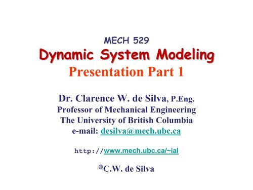
Dynamic System Modeling Presentation Part 1 - UBC Mechanical ...

MECH 529
Dynamic System Modeling
Presentation Part 1
Dr. Clarence W. de Silva, P.Eng.
Professor of Mechanical Engineering
The University of British Columbia
e-mail: desilva@mech.ubc.ca
http://www.mech.ubc.ca/~ial
©
C.W. de Silva

MECH 469/529: Modeling of Dynamic Systems; 3 Credits, 1st Term, 2012/13
Tuesdays and Thursdays (MacLeod 220), 5:00 to 6:30pm
Course Web Site: www.mech.ubc.ca/~ial (Courses MECH 529)
Instructor: Dr. Clarence W. de Silva, Professor
Office: CEME 2071; Telephone: 604-822-6291; e-mail: desilva@mech.ubc.ca
Teaching Assistant: Mr. Shawn Zhang
Office: ICICS 065; Tel: 604-822-4850; e-mail: yfzhang83@gmail.com
Prerequisites: This course is particularly suitable for senior undergraduate and entry-level
graduate engineering students. There are no specific prerequisites. But, students who have
already taken introductory courses in circuit analysis, dynamics, fluid mechanics, and
thermodynamics (or energy conversion) will be at an advantage.
Objectives
The course deals with the methodology of understanding and modeling a physical engineering
system. The primary emphasis will be on the engineering problem of modeling rather than the
applied mathematics of response analysis (and simulation) once a model is available.
The students will learn to understand and model mechanical, thermal, fluid and electrical
systems in a systematic and unified/integrated manner. For example, identification of lumped
elements such as sources, capacitors, inductors, and resistors in different types of physical
systems will be studied. Analogies among the four main types of systems (mechanical, thermal,
fluid and electrical) will be presented in terms of these basic lumped elements and in terms of the
system variables. Concepts of through and across variables, and flow and effort variables will be
introduced. Multi-domain (or mixed) systems which consist of two or more of the basic system
types will be considered as well.
Tools of modeling and model-representation such as linear graphs and block diagrams will be
discussed. Important considerations of input, output, causality, and system order will be examined.
Thevenin and Norton equivalent circuits and their application to mechanical systems using linear
graphs will be studied. A brief overview of response analysis will be given.
Textbook: de Silva, C.W., Modeling and Control of Engineering Systems, Taylor & Francis/CRC Press,
Boca Raton, FL, 2009.

MECH 469/529 COURSE LAYOUT
Week Starts Topic Read
1 Sept 06 Introduction Chapter 1
2 Sept 11 Model Types, Analogies Chapter 2
3 Sept 18 Electrical Systems Chapter 2
4 Sept 25 Fluid Systems Chapter 2
5 Oct 02 Thermal Systems Chapter 2
6 Oct 09 State-space Models Chapter 2
7 Oct 16 Model Linearization Chapter 3
8 Oct 23 Linear Graphs Chapter 4
9 Oct 30 State Models from Linear Graphs Chapter 4
10 Nov 06
Thursday, Nov 08:
Transfer Function Models
Intermediate Exam
Chapter 5
11 Nov 13 Thevenin/Norton Equivalent
Circuits; Linear Graph Reduction
Chapter 5
12 Nov 20 Simulation Block Diagrams; Chapter 6
13 Nov 27
Thursday, Nov 29:
Response Analysis and Simulation
Advanced Topics; Modeling
Applications
Final Take-home Exam Given Out
Monday, Dec 03: Final Take-home Exam Due
Grade Composition
Intermediate examination 40%
Attendance 10%
Final Exam (different for MECH 469 and MECH 529) 50%
Total 100%

Course Objectives
Methodology of understanding and modeling a physical
engineering dynamic system.
Primary Emphasis: Procedure of analytical modeling
Secondary: Response analysis and simulation once modeled
Systematic, Unified Approach to Modeling of:
mechanical, thermal, fluid, and electrical, systems
Analogies among these four types of systems
Multi-domain (Mixed) Systems: Have two or more basic
system types
Identification of Lumped Elements (sources, capacitors,
inductors, and resistors)
Through and Across Variables; Flow and Effort Variables
Systematic Tools of Modeling: Linear graphs, block diagrams
Important Considerations: Input, output, causality, system
order
Response Analysis and Simulation

Course Learning Activities
Power-point presentations will be posted on the web site
Assignments and solutions will be posted (not graded)
Past Exams and solutions will be posted
Office Hours: Mondays, 2:00 to 3:00 p.m. in CEME 2071
TA Office Hours: Thursdays, 3:30 to 4:30 p.m. in ICICS 065
November 08, 2012 (Thursday):
Intermediate Examination (In Class)
November 29, 2012 (Thursday):
Final Take-home Examination Given Out
December 03, 2012 (Monday):
Final Take-home Exam Due in Mech Office

Analytical Model Example:
Automated Gudeway Transit System

Analytical Model Example:
Automated Gudeway Transit System

Analytical Model Example:
Computer Hard Disk Drive (HDD)

Dynamic System
Environment
Dynamic System
(State Variables,
System Parameters)
Outputs/
Responses
Inputs/
Excitations
System
Boundary
Note: Rates of Changes of Outputs/State Variables are Not Negligible
(These rates are needed in the system representation)

TERMINOLOGY
System: Collection of interacting components of interest,
demarcated by a system boundary
Dynamic System: Rates of changes of response/state variables
(about some operating condition) cannot be neglected
Plant or Process: System to be controlled
Inputs: Excitations (known, unknown) to the system
Outputs: Responses of the system
State Variables: Completely identify the “dynamic” state of system
Note: If state variables at one state and inputs up to a future state
are known, the future state can be completely determined
Control System: Plant + controller, at least (May include sensors,
signal conditioning, etc.)

Examples of Dynamic Systems
System Typical Input Typical Outputs
Human body
Neuroelectric
pulses
Muscle contraction,
body movements
Company Information Decisions,
finished products
Power plant Fuel rate Electric power,
pollution rate
Automobile Steering wheel
movement
Front wheel turn,
direction of heading
Robot Voltage to joint Joint motions,
motor
effector motion

A DYNAMIC SYSTEM EXAMPLE:
A VISION-BASED WAFER INSPECTION Control System

A DYNAMIC SYSTEM EXAMPLE:
A MACHINE TOOL WHICH NEEDS ACCURATE CONTROL

It is a representation of a system
Dynamic Model
Useful in analysis, simulation, design, modification, and control
An engineering (e.g., Mechatronic) physical system consists of a
mixture of different types of components
An engineering (e.g., Mechatronic) system is typically a multidomain
(mixed) system
Integrated and unified development of model is desirable (i.e., all
domains are modeled together using similar approaches)
Use analogous procedures to model all components (in analytical
modeling)
Analogies exist in mechanical, electrical, fluid, and thermal
systems

MODEL TYPES
Model: A representation of a system.
Types of Models:
1. Physical Models (Prototypes)
2. Analytical Models
3. Computer (Numerical) Models (Data Tables, Curves, Programs,
Files, etc.)
4. Experimental Models (use input/output experimental data for
model “identification”)
Note:
Dynamic System: Response variables are functions of time,
with non-negligible rates of changes about an operating condition.

MODEL COMPLEXITY
• Universal Model (which considers all aspects of the system) is
unrealistic
E.g.: An automobile model that represents ride quality, energy
consumption, traction characteristics, handling, structural
strength, capacity, load characteristics, cost, safety, etc. is not
very practical
• Model may address a few specific aspects of
interest/application
• Model should be as simple as possible (Approximate
modeling, model reduction, etc. are applicable here)

ADVANTAGES OF ANALYTICAL MODELS
OVER PHYSICAL MODELS
• Modern, high-capacity, high-speed computers can accommodate
complex analytical models
• Models can be modified quickly, conveniently, and high speed at low
cost
• High flexibility of making structural and parametric changes
• Naturally amenable to computer simulations
• Can be integrated with computer/numerical/experimental models
• Can be done well before a prototype is built (and can be instrumental
in deciding whether to prototype)

ANALYTICAL MODEL TYPES
• Nonlinear: Nonlinear differential equations (principle of superposition does not hold)
• Linear: Linear differential equations (principle of superposition holds)
• Distributed (Continuous)-parameter: Partial differential equations (Dependent variables are
functions of time and space)
• Lumped-parameter: Ordinary differential equations (Dependent variables are functions of
time, not space)
• Time-varying (Non-stationary, Non-autonomous): Differential equations with time-varying
coefficients (Model parameters vary with time)
• Time-invariant (Stationary, Autonomous): Differential equations with constant coefficients
(Model parameters are constant)
• Random (Stochastic): Stochastic differential equations (Variables and/or parameters are
governed by probability distributions)
• Deterministic: Non-stochastic differential equations
• Continuous-time: Differential equations (Time variable is continuously defined)
• Discrete-time: Difference equations (Time variable is defined as discrete values at a sequence
of time points)

Lumped Model of a Distributed System: A Heavy Spring
Note: Mass (and flexibility) are distributed throughout the spring (not
at a few discrete points)

Lumped Model of a Distributed System: A Heavy Spring
m s = mass of spring; k = stiffness of spring; l = length of spring
One end fixed and the other end moving at velocity v
Kinetic Energy Equivalence
m
Local speed of element δx = x s
v. Element mass = δ x
l
Element kinetic energy KE =
l
l
1 m x s x(
v)
2 l
δ l
2
1 ms
x 1 msv
2 1 ms
As δx → dx, Total KE = ∫ dx(
v)
= x dx
3
2 l l 2 l
∫ =
2 3
0
2
l
2
2 v
Equivalent lumped mass concentrated at free end = 1 × spring mass
3
Assumption: Conditions are uniform along the spring.
0

Lumped Model of a Distributed System: A Heavy Spring
Lumped-parameter Approximation for an Oscillator with Heavy Spring

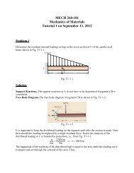
STEPS OF MODEL (ANALYTICAL) DEVELOPMENT
1. Identify system of interest (purpose, boundary)
2. Identify/specify variables of interest (excitations/inputs, responses/outputs, etc.)
3. Approximate various segments (processes, phenomena) by ideal elements, suitably
interconnected.
4. Draw a free-body or circuit diagram (or linear graph), with suitably isolated
components.
(a)Write constitutive equations (physical laws) for elements.
(b)Write continuity (or conservation) equations for
through variables (equilibrium of forces at joints; current balance at nodes, etc.)
(c)Write compatibility equations for across (potential or path) variables (loop
equations for velocities—geometric connectivity; voltages—potential balance)
(d)Eliminate auxiliary (unwanted) variables
5. Express boundary conditions and initial conditions using system variables.