Multifolded torus chaotic attractors: Design and implementation
Multifolded torus chaotic attractors: Design and implementation
Multifolded torus chaotic attractors: Design and implementation

You also want an ePaper? Increase the reach of your titles
YUMPU automatically turns print PDFs into web optimized ePapers that Google loves.
013118-3 <strong>Multifolded</strong> <strong>torus</strong> <strong>chaotic</strong> <strong>attractors</strong> Chaos 17, 013118 2007<br />
x<br />
9989 = y<br />
338 = z<br />
E S P<br />
P ± :<br />
−333<br />
corresponding to 1 <strong>and</strong> twodimensional<br />
unstable eigenspace E S P ± :−19865571x<br />
P<br />
+10076539y+9931196z=0 corresponding to 2,3 in the<br />
neighboring region of P ± .<br />
B. <strong>Design</strong> principles of system parameters<br />
Definition 1: An n-folded <strong>torus</strong> attractor is an attractor<br />
that is created via an n-<strong>torus</strong> breakdown route, where the<br />
n-<strong>torus</strong> is described as a quotient of R n under integral shifts<br />
in any coordinate with a zero Lyapunov number <strong>and</strong> an irrational<br />
rotation number. 8–10<br />
To generate multifolded <strong>torus</strong> <strong>chaotic</strong> <strong>attractors</strong> from the<br />
folded circuit 1, we introduce a new PWL odd function to<br />
replace the characteristic function 2, which is described by<br />
gy − x = m N−1 y − x<br />
N−1<br />
mi−1 − m<br />
+ <br />
i<br />
y − x + x i − y − x − x i , 3<br />
i=1 2<br />
where gx−y=−gy−x <strong>and</strong> , are real parameters.<br />
Note that the above PWL characteristic function gy−x<br />
can be recast as follows:<br />
y − x x 1 , m 0 y − x<br />
if x i y − x x i+1 , 1 i N −2,<br />
i<br />
gy − x =if<br />
m i y − x + m j−1 − m j sgny − xx j<br />
j=1<br />
N−1<br />
if y − x x n−1 , m N−1 y − x + m j−1 − m j sgny − xx j ,<br />
j=1<br />
4<br />
where m i 0iN−1 are the slopes of the segments, or<br />
radials in various piecewise subregions, <strong>and</strong> ±x i x i 0, 1<br />
iN−1 are the switching points. Since g· is an odd<br />
function, we only need to determine the positive switching<br />
points x i 1iN−1.<br />
Obviously, the equilibrium points of system 1 with 3<br />
are ±x i E ,0,0x i E 0,0iN−1, where ±x i E 0iN−1<br />
satisfies the following equation:<br />
gx i E =0, 0 i N −1. 5<br />
Substituting 4 into 5, <strong>and</strong> solving x E i 0iN−1 from<br />
5, yields the recursive formulas of x E i 0iN−1 as follows:<br />
= 0 i =0,<br />
x E i<br />
i j=1 m j − m j−1 x j<br />
6<br />
1 i N −1.<br />
m i<br />
Denote<br />
k i = x E<br />
i+1 − x i<br />
x E , 7<br />
i − x i<br />
E<br />
where 1iN−2. Let k i =1 for 1iN−2, thus x i<br />
= 1 2 x i+x i+1 for 1iN−2. That is, all internal equilibrium<br />
points x E i 0iN−2 are the midpoints of two neighboring<br />
switching points. According to 6, we have the recursive<br />
formulas of the positive switching points x i 2iN−1 as<br />
follows:<br />
x i+1 = 2 i<br />
j=1m j − m j−1 x j<br />
− x i , 8<br />
m i<br />
where 1iN−2.<br />
C. <strong>Multifolded</strong> <strong>torus</strong> <strong>chaotic</strong> <strong>attractors</strong><br />
Numerical simulation shows that system 1 with 3 has<br />
a large parameter region for chaos generation. Here, assume<br />
that =14.5, =1.25, <strong>and</strong> x 1 =0.75. Then, we can calculate<br />
all other switching points x i 2iN−1 from the recursive<br />
formulas 8.<br />
In the following, two typical cases are first discussed:<br />
N=2 <strong>and</strong> N=5. When N=2, we have gy−x=m 1 y−x<br />
+ 1 2 m 0−m 1 y−x+x 1 −y−x−x 1 . Let m 0 =0.15 <strong>and</strong> m 1<br />
=−0.17. Figure 2a shows the PWL characteristic function<br />
gx with N=2. For the above set of parameters, system 1<br />
with 3 has a 3-folded <strong>torus</strong> <strong>chaotic</strong> attractor, as shown in<br />
Fig. 3a. The maximum Lyapunov exponent of this 3-folded<br />
<strong>torus</strong> <strong>chaotic</strong> attractor is 0.1018. It is clear that there are three<br />
tori folded in the <strong>chaotic</strong> attractor, as shown in Fig. 3a.<br />
Obviously, system 1 with 3 for N=2 has three equilibrium<br />
points: O0,0,0 <strong>and</strong> P ± ±1.4118,0,0 denoted by “,”<br />
as shown in Fig. 3a. Also, the two switching points are<br />
denoted by “,” as shown in Fig. 3a.<br />
When N=5, we have<br />
gy − x = m 4 y − x<br />
4<br />
+ 2<br />
1 m i−1 − m i y − x + x i − y − x − x i .<br />
i=1<br />
Let m 0 =−0.17, m 1 =0.15, m 2 =−0.17, m 3 =0.15, <strong>and</strong> m 4 =<br />
−0.17. From 8, we have x 2 =2.45, x 3 =3.95, <strong>and</strong> x 4 =5.65.<br />
Figure 2b shows the PWL characteristic function gx for<br />
N=5. Here, system 1 with 3 has a 9-folded <strong>torus</strong> <strong>chaotic</strong><br />
attractor, as shown in Fig. 3b. The maximum Lyapunov<br />
exponent of this 9-folded <strong>torus</strong> <strong>chaotic</strong> attractor is 0.0730. It<br />
is clear that there are nine tori folded in the <strong>chaotic</strong> attractor,<br />
Downloaded 22 Mar 2007 to 144.214.40.14. Redistribution subject to AIP license or copyright, see http://chaos.aip.org/chaos/copyright.jsp