6 Coupled Oscillators

6
Coupled Oscillators
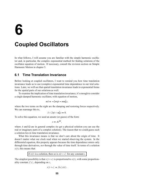
In what follows, I will assume you are familiar with the simple harmonic oscillator
and, in particular, the complex exponential method for finding solutions of the
oscillator equation of motion. If necessary, consult the revision section on Simple
Harmonic Motion in chapter 5.
0x=0: 0x;
6.1 Time Translation Invariance
Before looking at coupled oscillators, I want to remind you how time translation
invariance leads us to use (complex) exponential time dependence in our trial solutions.
Later, we will see that spatial translation invariance leads to exponential forms
for the spatial parts of our solutions as well.
To examine the implication of time translation invariance, it’s enough to consider
a single damped harmonic oscillator, with equation of motion,
mẍ=2mγẋmω 2
where the two terms on the right are the damping and restoring forces respectively.
We can rearrange this to,
ẍ+2γẋ+ω 2
To solve this equation, we used an ansatz (or guess) of the form
x(t+c)=f(c)x(t):
55
x=Ae Ωt;
where A and Ω are in general complex (to get a physical solution you can use the
real or imaginary parts of a complex solution). The reason that we could guess such
a solution lies in time translation invariance.
What this invariance means is that we don’t care about the origin of time. It
doesn’t matter what our clock read when we started observing the system. In the
differential equation, this property appears because the time dependence enters only
through time derivatives, not through the value of time itself. In terms of a solution
x(t), this means that:
if x(t)is a solution, then so is x(t+c)for any constant c.
The simplest possibility is that x(t+c)is proportional to x(t), with some proportionality
constant f(c), depending on c,

ẋ(t)=Ωx(t);
Ωt:
56 6 Coupled Oscillators
We can solve this equation by a simple trick. We differentiate with respect to c and
then set c=0to obtain
where Ω is just the value of ḟ(0). The general solution of this linear first order
differential equation is
x(t)=Ae
We often talk about complex exponential forms because Ω must have a non-zero
imaginary part if we want to get oscillatory solutions. In fact, from now on I will let
Ω=iω, so that ω is real for a purely oscillatory solution.
We can’t just use any value we like for ω. The allowed values are determined by
demanding that Ae iωt actually solves the equation of motion:
(ω 2+2iγω+ω
If we are to have a non-trivial solution, A should not vanish. The factor in parentheses
must then vanish, giving a quadratic equation to determine ω. The two roots of the
quadratic give us two independent solutions of the original second order differential
equation.
6.2 Normal Modes
n(t)):
We want to generalise from a single oscillator to a set of oscillators which can affect
each others’ motion. That is to say, the oscillators are coupled.
If there are n oscillators with positions x i(t)for i=1;:::;n , we will denote the
“position” of the whole system by a vector x(t)of the individual locations:
x(t)=(x 1(t);x 2(t);:::;x The individual positions x i(t)might well be generalised coordinates rather than real
physical positions.
The differential equations satisfied by the x i iωt;
will involve time dependence only
through time derivatives, which means we can look for a time translation invariant
solution, as described above. This means all the oscillators must have the same
complex exponential time dependence, e iωt , where ω is real for a purely oscillatory
motion. The solution then takes the form,
x(t)=0B@A 1
A 2
n1CAe .
A
where the A i are constants. This describes a situation where all the oscillators move
with the same frequency, but, in general, different phases and amplitudes: the oscillators’
displacements are in fixed ratios determined by the A i . This kind of motion
is called a normal mode. The overall normalisation is arbitrary (by linearity of the
differential equation), which is to say that you can multiply all the A i by the same
constant and still have the same normal mode.
Our job is to discover which ω are allowed, and then determine the set of A i
corresponding to each allowed ω. We will find precisely the right number of normal
modes to provide all the independent solutions of the set of differential equations.
For n oscillators obeying second order coupled equations there are 2n independent
2
0)Ae iωt=0:

6.3 Coupled Oscillators 57
solutions: we will find n coupled normal modes which will give us 2n real solutions
when we take the real and imaginary parts.
Once we have found all the normal modes, we can construct any possible motion
of the system as a linear combination of the normal modes. Compare this with
Fourier analysis, where any periodic function can be expanded as a series of sines
and cosines.
6.3 Coupled Oscillators
Take a set of coupled oscillators described by a set of coordinates q 1;:::;q n . In
general the potential V(q)will be a complicated function which couples all of these
oscillators together. Consider small oscillations about a position of stable equilibrium,
which (by redefining our coordinates if necessary) we can take to occur when
q i=0 for i=1;:::;n. Expanding the potential in a Taylor series about this point,
we find,
V(q)=V(0)+∑
∂V
q i+1
i
∂q i0 2 ∑ j0;
j+:
∂ 2 V
q i q
i;j
∂q i ∂q j0
By adding an overall constant to V we can choose V(0)=0. Since we are at a
position of equilibrium, all the first derivative terms vanish. So the first terms that
contribute are the second derivative ones. We define,
K i j∂2 V
∂q i ∂q
and drop all the remaining terms in the expansion. Note that K i j is a constant symmetric
(why?) nn matrix. The corresponding force
j;
is thus
F i=∂V
i=∑K i j q j
∂q
j
and thus the equations of motion are
K i j q
for i=1;:::;n. Here the M i are the masses of the oscillators, and K is a matrix of
‘spring constants’. Indeed for a system of masses connected by springs, with each
mass moving in the same single dimension, the coordinates can be taken as the real
position coordinates, and then M is a (diagonal in this case) matrix of masses, while
K is a matrix determined by the spring constants. Be aware however, that coupled
oscillator equations occur more generally (for example in electrical circuits) where
the q i s need not be actual coordinates but more general parameters describing the
system (known as generalised coordinates) and in this case M and K play similar
rôles even if they do not in actuality correspond to masses and spring constants.
To simplify the notation, we will write the equations of motion as a matrix equation.
So we define,
M=0B@M 1 1n
2n
.
. . .. . .
. . .. .
0 0M
M i ¨q i=∑
j
nn1CA:
00 n1CA;K=0B@K 11 K 12K 0 M 20
K 21 K 22K K n1 K n2K

k0
58 6 Coupled Oscillators
x 1 x 2
k1
m 1 m 2 k 2
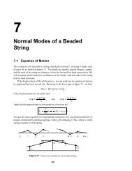
Figure 6.1 Two coupled harmonic oscillators. The vertical
n1CA:
dashed lines mark the equilibrium
positions of the two masses.
Likewise, let q and ¨q be column vectors,
q=0B@q 1
n1CA;¨q=0B@¨q
q 2
A:
1
¨q 2
.
.
q ¨q
With this notation, the equation of motion is,
M ¨q=Kq;or
Kq;
¨q=M1
where M1 is the inverse of M.
Now look for a normal mode solution, q=Ae iωt , where A is a column vector.
We have ¨q=ω 2 q, and cancelling e iωt factors, gives finally,
M1 KA=ω 2
This is now an eigenvalue equation. The squares of the normal mode freqencies are
the eigenvalues of M1 K, with the column vectors A as the corresponding eigenvectors.
6.4 Example: Masses and Springs
As a simple example, let’s look at the system shown in figure 6.1, comprising two
masses m 1 and m 2 constrained to move along a straight line. The masses are joined
by a spring with force constant k0, and m 1 (m 2 ) is joined to a fixed wall by a spring
with force constant k 1 (k 2 ). Assume that the equilibrium position of the system has
each spring unstretched, and use the displacements x 1 and x 2 of the two masses away
from their equilibrium positions as coordinates. The force on mass m 1 is then
F 1=k 1 x 1k0(x 1+k0k0 1): 2) 1x 2 x 2k0(x 2x (Note that these follow from a potential of form V=1
2 k 1x 2 1+1
2 k0(x 2x 1)2+1
2 k 2x 2 2 .)
You can check that Newton’s 2nd law thus implies, in matrix form:
2:
1
2=k 2+k0x 1
ẍ k0k x
The eigenvalue equation we have to solve is:
2A 1 2A 2=ω 1
k0=m 2(k A A
and on mass m 2
F 2=k
m 1 0
2ẍ
0 m
(k 1+k0)=m 1k0=m 1
2+k0)=m

2;
6.4 Example: Masses and Springs 25λ+4=0;
59
Now specialise to a case where m 1=m, m 2=2m,
0:
k 1=k, k 2=2k and k0=2k.
The eigenvalue equation becomes,
32
2A 1
2=m
ω2A 1
1 A k A
or, setting λ=mω 2=k,3λ2
2λA 1
2=0
1 A
For there to be a solution, the determinant of the 22 matrix in the last equation
must vanish. This gives a quadratic equation for λ,
λ
with roots λ=1 and λ=4. The corresponding eigenfrequencies are ω=pk=m
and ω=2pk=m. For each eigenvalue, there is a corresponding eigenvector. With
λ=1you find A 2=A m;
1 , and with λ=4 you find A 2=A 1;
1=2. Note that just the
ratio of the two A i is determined: you can multiply all the A i by a constant and stay
in the same normal mode. This means that we are free to normalise the eigenvectors
as we choose. It is common to make them have unit modulus, in which case the
eigenfrequencies and eigenvectors are:
A=1p21
ω=2rk
m; A=1p521;
ω=rk
In the first normal mode, the two masses swing in phase with the same amplitude,
and the middle spring remains unstretched. This could have been predicted: we have
solved for a case where m 2 is twice the mass of m 1 , and is attached to a wall by a
spring with twice the force constant. Therefore, m 1 and m 2 would oscillate with the
same frequency in the absence of the connecting spring.
In the second mode the two masses move out of phase with each other, and m 1
has twice the amplitude of m 2 .
6.4.1 Weak Coupling
m;
and Beats
Now consider a case where the two masses are equal, m 1=m 2=m, and the two
springs attaching the masses to the fixed
m; walls are identical, k
1;
1=k 2=k. From the
symmetry of the setup, you expect one mode where the two masses swing in phase
with the same amplitude, the central connecting spring remaining unstretched. In
the second mode, the two masses again have the same amplitude, but swing out of
phase, alternately approaching and receding from each other. This second mode will
have a higher frequency (why?).
If the spring constant of the connecting spring is k0=εk, you should check that
applying the solution method worked through above gives the following eigenfrequencies
and normal modes:
A 1=1p21
A 2=1p21
1=rk
ω
2=r(1+2ε)k
ω

60 6 Coupled Oscillators
0;
t):
When the connecting spring has a very small force constant, ε1, so that the
coupling is weak, the two normal modes have almost the same frequency. In this
case it’s possible to observe beats when a motion contains components from both
normal modes. For example, suppose you start the system from rest by holding the
left hand mass with a small displacement to the right, say d, keeping the right hand
mass in its equilibrium position, and then letting go.
A general solution for the motion has the form,
2 A 2 cos(ω 2 t)+c 3 A 1
1;
sin(ω 1 t)+c 4 A 2 sin(ω 2
Because the system starts from rest, you can immediately see (make sure you can!)
that c 3=c 4=0in
t));
this case. Then the initial condition,
x(0)=d
gives, d
0=c p21 1
1+c p21 2
t)):
which is solved by c 1=c 2=d=p2. So, the motion is given by:
1(t)=d
x 1 t)+cos(ω 2
2(cos(ω 2(t)=d
t: t;
x 1 t)cos(ω 2
2(cos(ω We can rewrite the sum and difference of cosines as products, leaving:
2ω x cosω
1(t)=d 1
1+ω 2
tcosω
2
2
2ω x sinω
2(t)=d 1
1+ω 2
tsinω
2
2
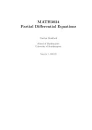
Now you can see that each of x 1 and x 2 has a “fast” oscillation at the average frequency(ω
1+ω 2)=2, modulated by a “slow” amplitude variation at the difference
frequency(ω 2ω 1)=2. The displacements show the contributions of the two normal
modes beating together, as illustrated in figure 6.2.
You can easily demonstrate beats by tying a length of cotton between two chairs
and hanging two keys from it by further equal-length threads. Each key is a simple
pendulum and the suspension thread provides a weak coupling between them. Start
the system by pulling one of the keys to one side, with the other hanging vertically,
and releasing, so that you start with one key swinging from side to side and the
other at rest. The swinging key gradually reduces its amplitude, and at the same
time the other key begins to move. Eventually, the first key will momementarily
stop swinging, whilst the second key has reached full amplitude. The process then
continues, and the swinging motion transfers back and forth between the two keys.
x(t)=c 1 A 1 cos(ω 1 t)+c

6.4 Example: Masses and Springs 61
1(t) x
2(t) x
d
d
5 10 15 20
ω 1 t
2π
d
5 10 15 20
ω 1 t
2π
d
Figure 6.2 Displacements x 1 and x 2 as functions of time, starting with both masses at rest
and x 1(0)=d, x 2(0)=0. The displacement curve for x 2 is shown dashed. For this plot, the
ratio ε of the spring force constants of the coupling (central) spring and either of the outer
springs is 0:1. Time is plotted in units of the period of the lower frequency normal mode.

62 6 Coupled Oscillators