Panel Data Analysis, Josef Brüderl - Sowi
Panel Data Analysis, Josef Brüderl - Sowi
Panel Data Analysis, Josef Brüderl - Sowi

Create successful ePaper yourself
Turn your PDF publications into a flip-book with our unique Google optimized e-Paper software.
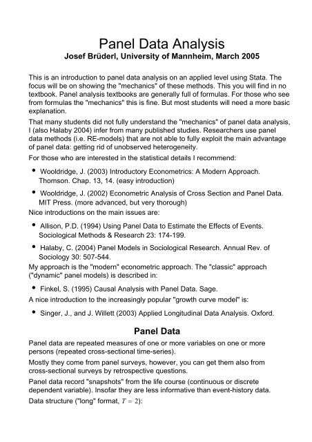
<strong>Panel</strong> <strong>Data</strong> <strong>Analysis</strong><br />
<strong>Josef</strong> Brüderl, University of Mannheim, March 2005<br />
This is an introduction to panel data analysis on an applied level using Stata. The<br />
focus will be on showing the "mechanics" of these methods. This you will find in no<br />
textbook. <strong>Panel</strong> analysis textbooks are generally full of formulas. For those who see<br />
from formulas the "mechanics" this is fine. But most students will need a more basic<br />
explanation.<br />
That many students did not fully understand the "mechanics" of panel data analysis,<br />
I (also Halaby 2004) infer from many published studies. Researchers use panel<br />
data methods (i.e. RE-models) that are not able to fully exploit the main advantage<br />
of panel data: getting rid of unobserved heterogeneity.<br />
For those who are interested in the statistical details I recommend:<br />
• Wooldridge, J. (2003) Introductory Econometrics: A Modern Approach.<br />
Thomson. Chap. 13, 14. (easy introduction)<br />
• Wooldridge, J. (2002) Econometric <strong>Analysis</strong> of Cross Section and <strong>Panel</strong> <strong>Data</strong>.<br />
MIT Press. (more advanced, but very thorough)<br />
Nice introductions on the main issues are:<br />
• Allison, P.D. (1994) Using <strong>Panel</strong> <strong>Data</strong> to Estimate the Effects of Events.<br />
Sociological Methods & Research 23: 174-199.<br />
• Halaby, C. (2004) <strong>Panel</strong> Models in Sociological Research. Annual Rev. of<br />
Sociology 30: 507-544.<br />
My approach is the "modern" econometric approach. The "classic" approach<br />
("dynamic" panel models) is described in:<br />
• Finkel, S. (1995) Causal <strong>Analysis</strong> with <strong>Panel</strong> <strong>Data</strong>. Sage.<br />
A nice introduction to the increasingly popular "growth curve model" is:<br />
• Singer, J., and J. Willett (2003) Applied Longitudinal <strong>Data</strong> <strong>Analysis</strong>. Oxford.<br />
<strong>Panel</strong> <strong>Data</strong><br />
<strong>Panel</strong> data are repeated measures of one or more variables on one or more<br />
persons (repeated cross-sectional time-series).<br />
Mostly they come from panel surveys, however, you can get them also from<br />
cross-sectional surveys by retrospective questions.<br />
<strong>Panel</strong> data record "snapshots" from the life course (continuous or discrete<br />
dependent variable). Insofar they are less informative than event-history data.<br />
<strong>Data</strong> structure ("long" format, T 2):
<strong>Panel</strong> <strong>Data</strong> <strong>Analysis</strong>, <strong>Josef</strong> Brüderl 2<br />
i t y x<br />
1 1 y 11 x 11<br />
1 2 y 12 x 12<br />
2 1 y 21 x21<br />
2 2 y 22 x22<br />
<br />
N 1 y N1 x N1<br />
N 2 y N2 xN2<br />
Benefits of panel data:<br />
• They are more informative (more variability, less collinearity, more degrees of<br />
freedom), estimates are more efficient.<br />
• They allow to study individual dynamics (e.g. separating age and cohort<br />
effects).<br />
• They give information on the time-ordering of events.<br />
• They allow to control for individual unobserved heterogeneity.<br />
Since unobserved heterogeneity is the problem of non-experimental research, the<br />
latter benefit is especially useful.<br />
<strong>Panel</strong> <strong>Data</strong> and Causal Inference<br />
According to the counterfactual approach on causality (Rubin’s model), the causal<br />
effect of a treatment (T) is defined by (individual i, time t 0 , before treatment C):<br />
T<br />
Y i,t0<br />
− Y C i,t0 .<br />
This obviously is not estimable. With cross-sectional data we estimate (between<br />
estimation)<br />
T<br />
Y i,t0<br />
− Y C j,t0 .<br />
This only provides the true causal effect if the assumption of unit homogeneity (no<br />
unobserved heterogeneity) holds. With panel data we can improve on this, by using<br />
(within estimation)<br />
T<br />
Y i,t1<br />
− Y C i,t0 .<br />
Unit homogeneity here is needed only in an intrapersonal sense! However, period<br />
effects might endanger causal inference. To avoid this, we could use<br />
(difference-in-differences estimator)<br />
T<br />
Y i,t1<br />
− Y C i,t0 − Y C<br />
j,t1<br />
− Y C j,t0 .
<strong>Panel</strong> <strong>Data</strong> <strong>Analysis</strong>, <strong>Josef</strong> Brüderl 3<br />
Example: Does marriage increase the wage of men?<br />
Many cross-sectional studies have shown that married men earn more. But is this<br />
effect causal? Probably not. Due to self-selection this effect might be spurious.<br />
High-ability men select themselves (or are selected) into marriage. In addition, high<br />
ability-men earn more. Since researchers usually have no measure of ability, there<br />
is potential for an omitted variable bias (unobserved heterogeneity).<br />
I have constructed an artificial dataset, where there is both selectivity and a causal<br />
effect:<br />
. list id time wage marr, separator(6)<br />
------------------------- -------------------------<br />
| id time wage marr | | id time wage marr |<br />
|-------------------------| |-------------------------|<br />
1. | 1 1 1000 0 | 13. | 3 1 2900 0 |<br />
2. | 1 2 1050 0 | 14. | 3 2 3000 0 |<br />
3. | 1 3 950 0 | 15. | 3 3 3100 0 |<br />
4. | 1 4 1000 0 | 16. | 3 4 3500 1 |<br />
5. | 1 5 1100 0 | 17. | 3 5 3450 1 |<br />
6. | 1 6 900 0 | 18. | 3 6 3550 1 |<br />
|-------------------------| |-------------------------|<br />
7. | 2 1 2000 0 | 19. | 4 1 3950 0 |<br />
8. | 2 2 1950 0 | 20. | 4 2 4050 0 |<br />
9. | 2 3 2000 0 | 21. | 4 3 4000 0 |<br />
10. | 2 4 2000 0 | 22. | 4 4 4500 1 |<br />
11. | 2 5 1950 0 | 23. | 4 5 4600 1 |<br />
12. | 2 6 2100 0 | 24. | 4 6 4400 1 |<br />
|-------------------------| -------------------------<br />
We observe four men (N 4) for six years (T 6). Wage varies a little around<br />
1000, 2000, 3000, and 4000 € respectively. The two high-wage men marry between<br />
year 3 and 4 (selectivity). This is indicated by "marr" jumping from 0 to 1. (This<br />
specification implies a lasting effect of marriage).<br />
Note that with panel data we have two sources of variation: between and within<br />
persons.<br />
twoway<br />
(scatter wage time, ylabel(0(1000)5000, grid)<br />
ymtick(500(1000)4500, grid) c(L))<br />
(scatter wage time if marr1, c(L)),<br />
legend(label(1 "before marriage") label(2 "after marriage"))
<strong>Panel</strong> <strong>Data</strong> <strong>Analysis</strong>, <strong>Josef</strong> Brüderl 4<br />
EURO per month<br />
0 1000 2000 3000 4000 5000<br />
1 2 3 4 5 6<br />
Time<br />
before marriage<br />
after marriage<br />
Identifying the Marriage Effect<br />
Now, what is the effect of marriage in these data? Clearly there is self-selection: the<br />
high-wage men marry. In addition, however, there is a causal effect of marriage:<br />
After marriage there is a wage increase (whereas there is none, for the "control<br />
group").<br />
More formally, we use the difference-in-differences (DID) approach. First, compute<br />
for every man the mean wage before and after marriage (for unmarried men before<br />
year 3.5 and after). Then, compute for every man the difference in the mean wage<br />
before and after marriage (before-after difference). Take the average of married<br />
and unmarried men. Finally, the difference of the before-after difference of married<br />
and unmarried men is the causal effect:<br />
4500 − 4000 3500 − 3000<br />
2<br />
−<br />
2000 − 2000 1000 − 1000<br />
2<br />
500.<br />
In this example, marriage causally increases earnings by 500 €. (At least this is<br />
what I wanted it to be, but due to a "data construction error" the correct<br />
DID-estimator is 483 €. Do you find the "error"?).<br />
The DID-approach mimics what one would do with experimental data. In identifying<br />
the marriage effect we rely on a within-person comparison (the before-after<br />
difference). To rule out the possibility of maturation or period effects we compare<br />
the within difference of married (treatment) and unmarried (control) men.<br />
The Fundamental Problem of Non-Experimental Research<br />
What would be the result of a cross-sectional regression at T 4<br />
y i4 0 1 x i4 u i4 ?
<strong>Panel</strong> <strong>Data</strong> <strong>Analysis</strong>, <strong>Josef</strong> Brüderl 5<br />
<br />
1<br />
2500 (this is the difference of the wage mean between married and unmarried<br />
men). The estimate is highly misleading!<br />
It is biased because of unobserved heterogeneity (also called: omitted variables<br />
bias): unobserved ability is in the error term, therefore u i4 and x i4 are correlated.<br />
The central regression assumption is, however, that the X-variable and the error<br />
term are uncorrelated (exogeneity). Endogeneity (X-variable correlates with the<br />
error term) results in biased regression estimates. Endogeneity is the fundamental<br />
problem of non-experimental research. Endogeneity can be the consequence of<br />
three mechanisms: unobserved heterogeneity (self-selection), simultaneity, and<br />
measurement error (for more on this see below).<br />
The nature of the problem can be seen in the Figure from above: the<br />
cross-sectional OLS estimator relies totally on a between-person comparison. This<br />
is misleading because persons are self-selected. In an experiment we would assign<br />
persons randomly.<br />
With cross-sectional data we could improve on this only, if we would have<br />
measured "ability". In the absence of such a measure our conclusions will be<br />
wrong. Due to the problem of unobserved heterogeneity the results of many<br />
cross-sectional studies are highly disputable.<br />
What to Do?<br />
The best thing would be to conduct an experiment. If this is not possible collect at<br />
least longitudinal data. As we saw above, with panel data it is possible to identify<br />
the true effect, even in the presence of self-selection!<br />
In the following, we will discuss several regression methods for panel data. The<br />
focus will be on showing, how these methods succeed in identifying the true causal<br />
effect. We will continue with the data from our artificial example.<br />
Pooled-OLS<br />
We pool the data and estimate an OLS regression (pooled-OLS)<br />
y it 0 1 x it u it .<br />
<br />
1<br />
1833 (the mean of the red points minus the mean of the green points). This<br />
estimate is still heavily biased because of unobserved heterogeneity (u it and x it are<br />
correlated). This is due to the fact that pooled-OLS also relies on a between<br />
comparison. Compared with the cross-sectional OLS the bias is lower, however,<br />
because pooled-OLS also takes regard of the within variation.<br />
Thus, panel data alone do not remedy the problem of unobserved heterogeneity!<br />
One has to apply special regression models.
<strong>Panel</strong> <strong>Data</strong> <strong>Analysis</strong>, <strong>Josef</strong> Brüderl 6<br />
Error-Components Model<br />
These regression models are based on the following modelling strategy. We<br />
decompose the error term in two components: A person-specific error i and an<br />
idiosyncratic error it ,<br />
u it i it .<br />
The model is now (we omit the constant, because it would be collinear with i ):<br />
y it 1 x it i it .<br />
The person-specific error does not change over time. Every person has a fixed<br />
value on this latent variable (fixed-effects). i represents person-specific<br />
time-constant unobserved heterogeneity. In our example i could be unobserved<br />
ability (which is constant over the six years).<br />
The idiosyncratic error varies over individuals and time. It should fulfill the<br />
assumptions for standard OLS error terms.<br />
The assumption of pooled-OLS is that x it is uncorrelated both with i and it .<br />
First-Difference Estimator<br />
With panel data we can "difference out" the person-specific error (T 2):<br />
y i2 1 x i2 i i2<br />
y i1 1 x i1 i i1 .<br />
Subtracting the second equation from the first gives:<br />
Δy i 1 Δx i Δ i ,<br />
where "Δ" denotes the change from t 1 to t 2. This is a simple cross-sectional<br />
regression equation in differences (without constant). 1 canbeestimated<br />
consistently by OLS, if it is uncorrelated with x it (first-difference (FD) estimator).<br />
The big advantage is that the fixed-effects have been cancelled out. Therefore, we<br />
no longer need the assumption that i is uncorrelated with x it . Time-constant<br />
unobserved heterogeneity is no longer a problem.<br />
Differencing is also straightforward with more than two time-periods. For T 3 one<br />
could subtract period 1 from 2, and period 2 from 3. This estimator, however, is not<br />
efficient, because one could also subtract period 1 from 3 (this information is not<br />
used). In addition, with more than two time-periods the problem of serially<br />
correlated Δ i arises. OLS assumes that error terms across observations are<br />
uncorrelated (no autocorrelation). This assumption can easily be violated with<br />
multi-period panel data. Then S.E.s will be biased. To remedy this one can use<br />
GLS or Huber-White sandwich estimators.
<strong>Panel</strong> <strong>Data</strong> <strong>Analysis</strong>, <strong>Josef</strong> Brüderl 7<br />
Example<br />
We generate the first-differenced variables:<br />
tsset id time<br />
/* tsset the data<br />
generate dwage wage - L.wage /* L. is the lag-operator<br />
generate dmarr marr - L.marr<br />
Then we run an OLS regression (with no constant):<br />
. regress dwage dmarr, noconstant<br />
Source | SS df MS Number of obs 20<br />
--------------------------------------- F( 1, 19) 39.46<br />
Model | 405000 1 405000 Prob F 0.0000<br />
Residual | 195000 19 10263.1579 R-squared 0.6750<br />
--------------------------------------- Adj R-squared 0.6579<br />
Total | 600000 20 30000 Root MSE 101.31<br />
-----------------------------------------------------------------------<br />
dwage | Coef. Std. Err. t P|t| [95% Conf. Interval]<br />
----------------------------------------------------------------------<br />
dmarr | 450 71.63504 6.28 0.000 300.0661 599.9339<br />
-----------------------------------------------------------------------<br />
Next with robust S.E. (Huber-White sandwich estimator):<br />
. regress dwage dmarr, noconstant cluster(id)<br />
Regression with robust standard errors Number of obs 20<br />
F( 1, 3) 121.50<br />
Prob F 0.0016<br />
R-squared 0.6750<br />
Number of clusters (id) 4 Root MSE 101.31<br />
-----------------------------------------------------------------------<br />
| Robust<br />
dwage | Coef. Std. Err. t P|t| [95% Conf. Interval]<br />
----------------------------------------------------------------------<br />
dmarr | 450 40.82483 11.02 0.002 320.0772 579.9228<br />
-----------------------------------------------------------------------<br />
We see that the FD-estimator identifies the true causal effect (almost). Note that the<br />
robust S.E. is much lower.<br />
However, the FD-estimator is inefficient because it uses only the wage observations<br />
immediately before and after a marriage to estimate the slope (i.e., two<br />
observations!). This can be seen in the following plot of the first-differenced data:<br />
twoway<br />
(scatter dwage dmarr)<br />
(lfit dwage dmarr, estopts(noconstant)),<br />
legend(off) ylabel(-200(100)600, grid)<br />
xtitle(delta(marr)) ytitle(delta(wage));
<strong>Panel</strong> <strong>Data</strong> <strong>Analysis</strong>, <strong>Josef</strong> Brüderl 8<br />
delta(wage)<br />
-200 -100 0 100 200 300 400 500 600<br />
0 .2 .4 .6 .8 1<br />
delta(marr)<br />
Within-person change<br />
The intuition behind the FD-estimator is that it no longer uses the between-person<br />
comparison. It uses only within-person changes: If X changes, how much does Y<br />
change (within one person)? Therefore, in our example, unobserved ability<br />
differences between persons no longer bias the estimator.<br />
Fixed-Effects Estimation<br />
An alternative to differencing is the within transformation. We start from the<br />
error-components model:<br />
y it 1 x it i it .<br />
Average this equation over time for each i (between transformation):<br />
y i<br />
1 x i i i .<br />
Subtract the second equation from the first for each t (within transformation):<br />
y it − y i<br />
1 x it − x i it − i .<br />
This model can be estimated by pooled-OLS (fixed-effects (FE) estimator). The<br />
important thing is that again the i have disappeared. We no longer need the<br />
assumption that i is uncorrelated with x it . Time-constant unobserved heterogeneity<br />
is no longer a problem.<br />
What we do here is to "time-demean" the data. Again, only the within variation is<br />
left, because we subtract the between variation. But here all information is used, the<br />
within transformation is more efficient than differencing. Therefore, this estimator is<br />
also called the within estimator.<br />
Example<br />
We time-demean our data and run OLS:<br />
egen<br />
mwage mean(wage), by(id)
<strong>Panel</strong> <strong>Data</strong> <strong>Analysis</strong>, <strong>Josef</strong> Brüderl 9<br />
egen mmarr mean(marr), by(id)<br />
generate wwage wage - mwage<br />
generate wmarr marr - mmarr<br />
. regress wwage wmarr<br />
Source | SS df MS Number of obs 24<br />
------------------------------------- F( 1, 22) 183.33<br />
Model | 750000 1 750000 Prob F 0.0000<br />
Resid | 90000 22 4090.90909 R-squared 0.8929<br />
------------------------------------- Adj R-squared 0.8880<br />
Total | 840000 23 36521.7391 Root MSE 63.96<br />
----------------------------------------------------------------------<br />
wwage | Coef. Std. Err. t P|t| [95% Conf. Interval]<br />
---------------------------------------------------------------------<br />
wmarr | 500 36.92745 13.54 0.000 423.4172 576.5828<br />
_cons | 0 13.05582 0.00 1.000 -27.07612 27.07612<br />
----------------------------------------------------------------------<br />
The FE-estimator succeeds in identifying the true causal effect! However, OLS uses<br />
df N T − k. This is wrong, since we used up another N degrees of freedom by<br />
time-demeaning. Correct is df N T − 1 − k. xtreg takes regard of this (and<br />
demeans automatically):<br />
. xtreg wage marr, fe<br />
Fixed-effects (within) regression Number of obs 24<br />
Group variable (i): id Number of groups 4<br />
R-sq: within 0.8929 Obs per group: min 6<br />
between 0.8351 avg 6.0<br />
overall 0.4064 max 6<br />
F(1,19) 158.33<br />
corr(u_i, Xb) 0.5164 Prob F 0.0000<br />
----------------------------------------------------------------------<br />
wage | Coef. Std. Err. t P|t| [95% Conf. Interval]<br />
---------------------------------------------------------------------<br />
marr | 500 39.73597 12.58 0.000 416.8317 583.1683<br />
cons | 2500 17.20618 145.30 0.000 2463.987 2536.013<br />
---------------------------------------------------------------------<br />
sigma_u | 1290.9944<br />
sigma_e | 68.82472<br />
rho | .99716595 (fraction of variance due to u_i)<br />
----------------------------------------------------------------------<br />
F test that all u_i0: F(3, 19) 1548.15 Prob F 0.0000<br />
The S.E. is somewhat larger. R 2 -within is the explained variance for the demeaned<br />
data. This is the one that you would want to report. sigma_u is and sigma_e is<br />
. By construction of our dataset the estimated person-specific error is much<br />
larger. (There is a constant in the output, because Stata after the within<br />
transformation adds back the overall wage mean, which is 2500 €.)<br />
An intuitive feeling for what the FE-estimator does, gives this plot:<br />
twoway<br />
(scatter wwage wmarr, jitter(2))<br />
(lfit wwage wmarr),<br />
legend(off) ylabel(-400(100)400, grid)<br />
xtitle(demeaned(marr)) ytitle(demeaned(wage));
<strong>Panel</strong> <strong>Data</strong> <strong>Analysis</strong>, <strong>Josef</strong> Brüderl 10<br />
demeaned(wage)<br />
-400 -300 -200 -100 0 100 200 300 400<br />
-.5 0 .5<br />
demeaned(marr)<br />
All wage observations of those who married contribute to the slope of the<br />
FE-regression. Basically, it compares the before-after wages of those who married.<br />
However, it does not use the observations of the "control-group" (those, who did not<br />
marry). These are at X 0 and contribute nothing to the slope of the FE-regression.<br />
Dummy Variable Regression (LSDV)<br />
Instead of demeaning the data, one could include a dummy for every i and estimate<br />
the first equation from above by pooled-OLS<br />
(least-squares-dummy-variables-estimator). This provides also the FE-estimator<br />
(with correct test statistics)! In addition, we get estimates for the i which may be of<br />
substantive interest.<br />
. tabulate id, gen(pers)<br />
. regress wage marr pers1-pers4, noconstant<br />
Source | SS df MS Number of obs 24<br />
--------------------------------------- F( 5, 19) 8550.00<br />
Model | 202500000 5 40500000 Prob F 0.0000<br />
Residual | 90000 19 4736.84211 R-squared 0.9996<br />
--------------------------------------- Adj R-squared 0.9994<br />
Total | 202590000 24 8441250 Root MSE 68.825<br />
----------------------------------------------------------------------<br />
wage | Coef. Std. Err. t P|t| [95% Conf. Interval]<br />
---------------------------------------------------------------------<br />
marr | 500 39.73597 12.58 0.000 416.8317 583.1683<br />
pers1 | 1000 28.09757 35.59 0.000 941.1911 1058.809<br />
pers2 | 2000 28.09757 71.18 0.000 1941.191 2058.809<br />
pers3 | 3000 34.41236 87.18 0.000 2927.974 3072.026<br />
pers4 | 4000 34.41236 116.24 0.000 3927.974 4072.026<br />
----------------------------------------------------------------------<br />
The LSDV-estimator, however, is practical only when N is small.<br />
Individual Slope Regressions<br />
Another way to obtain the FE-estimator is to estimate a regression for every
<strong>Panel</strong> <strong>Data</strong> <strong>Analysis</strong>, <strong>Josef</strong> Brüderl 11<br />
individual (this is a kind of "random- coefficient model"). The mean of the slopes is<br />
the FE-estimator.<br />
Our example: The slopes for the two high-wage men are 500. The regressions for<br />
the two low-wage men are not defined, because X does not vary (again we see that<br />
the FE-estimator does not use the "control group"). That means, the FE-estimator is<br />
500, the true causal effect.<br />
With spagplot (an Ado-file you can net search) it is easy to produce a plot with<br />
individual regression lines (the red curve is pooled-OLS). This is called a "spaghetti<br />
plot":<br />
spagplot wage marr if id2, id(id) ytitle("EURO per month") xlabel(0 1)<br />
ylabel(0(1000)5000, grid) ymtick(500(1000)4500, grid) note("")<br />
EURO per month<br />
0 1000 2000 3000 4000 5000<br />
0 1<br />
marriage<br />
Such a plot shows nicely, how much pooled-OLS is biased, because it uses also<br />
the between variation.<br />
Restrictions<br />
1. With FE-regressions we cannot estimate the effects of time-constant<br />
covariates. These are all cancelled out by the within transformation. This<br />
reflects the fact that panel data do not help to identify the causal effect of a<br />
time-constant covariate (estimates are only more efficient)! The "within logic"<br />
applies only with time-varying covariates.<br />
2. Further, there must be some variation in X. Otherwise, we cannot estimate its<br />
effect. This is a problem, if only a few observations show a change in X. For<br />
instance, estimating the effect of education on wages with panel data is<br />
difficult. Cross-sectional education effects are likely to be biased (ability bias).<br />
<strong>Panel</strong> methods would be ideal (cancelling out the unobserved fixed ability<br />
effect). But most workers show no change in education. The problem will show<br />
up in a huge S.E.<br />
Random-Effects Estimation<br />
Again we start from the error-components model (now with a constant)
<strong>Panel</strong> <strong>Data</strong> <strong>Analysis</strong>, <strong>Josef</strong> Brüderl 12<br />
y it 0 1 x it i it .<br />
Now it is assumed that the i are random variables (i.i.d. random-effects) and that<br />
Covx it , i 0. Then we obtain consistent estimates by using pooled-OLS.<br />
However, we have now serially correlated error terms u it , and S.E.s are biased.<br />
Using a pooled-GLS estimator provides the random-effects (RE) estimator.<br />
It can be shown that the RE-estimator is obtained by applying pooled-OLS to the<br />
data after the following transformation:<br />
y it − y i<br />
0 1 − 1 x it − x i 1 − i it − i ,<br />
where<br />
1 −<br />
<br />
2<br />
T 2 <br />
2 .<br />
If 1 the RE-estimator is identical with the FE-estimator. If 0 the RE-estimator<br />
is identical with the pooled OLS-estimator. Normally will be between 0 and 1. The<br />
RE-estimator mixes within and between estimators! If Covx it , i 0 this is ok, it<br />
even increases efficiency. But if Covx it , i ≠ 0 the RE-estimator will be biased. The<br />
degree of the bias will depend on the magnitude of . If 2 2 then will be close<br />
to 1, and the bias of the RE-estimator will be low.<br />
Example<br />
. xtreg wage marr, re theta<br />
Random-effects GLS regression Number of obs 24<br />
Group variable (i): id Number of groups 4<br />
R-sq: within 0.8929 Obs per group: min 6<br />
between 0.8351 avg 6.0<br />
overall 0.4064 max 6<br />
Random effects u_i ~Gaussian Wald chi2(1) 121.76<br />
corr(u_i, X) 0 (assumed) Prob chi2 0.0000<br />
theta .96026403<br />
-----------------------------------------------------------------------<br />
wage | Coef. Std. Err. z P|z| [95% Conf. Interval]<br />
----------------------------------------------------------------------<br />
marr | 503.1554 45.59874 11.03 0.000 413.7835 592.5273<br />
_cons | 2499.211 406.038 6.16 0.000 1703.391 3295.031<br />
----------------------------------------------------------------------<br />
sigma_u | 706.54832<br />
sigma_e | 68.82472<br />
rho | .99060052 (fraction of variance due to u_i)<br />
-----------------------------------------------------------------------<br />
The RE-estimator works quite well. The bias is only 3. This is because<br />
1 − 68. 8 2<br />
6 706. 5 2 68. 8 2 0. 96.<br />
The option theta includes the estimate in the output.<br />
One could use a Hausman specification test on whether the RE-estimator is biased.
<strong>Panel</strong> <strong>Data</strong> <strong>Analysis</strong>, <strong>Josef</strong> Brüderl 13<br />
This test, however, is based on strong assumptions which are usually not met in<br />
finite samples. Often it does even not work (as with our data).<br />
FE- or RE-Modelling?<br />
1. For most research problems one would suspect that Covx it , i ≠ 0. The<br />
RE-estimator will be biased. Therefore, one should use the FE-estimator to get<br />
unbiased estimates.<br />
2. The RE-estimator, however, provides estimates for time-constant covariates.<br />
Many researchers want to report effects of sex, race, etc. Therefore, they<br />
choose the RE-estimator over the FE-estimator. In most applications, however,<br />
the assumption Covx it , i 0 will be wrong, and the RE-estimator will be<br />
biased (though the magnitude of the bias could be low). This is risking to throw<br />
away the big advantage of panel data only to be able to write a paper on "The<br />
determinants of Y". To take full advantage of panel data the style of data<br />
analysis has to change: One should concentration on the effects of (a few)<br />
time-varying covariates only and use the FE-estimator consequently!<br />
3. The RE-estimator is a special case of a parametric model for unobserved<br />
heterogeneity: We make distributional assumptions on the person-specific<br />
error term and conceive an estimation method that cancels the nuisance<br />
parameters. Generally, such models do not succeed in solving the problem of<br />
unobserved heterogeneity! In fact, they work only if there is "irrelevant"<br />
unobserved heterogeneity: Covx it , i 0.<br />
Further Remarks on <strong>Panel</strong>-Regression<br />
1. Though it is not possible to include time-constant variables in a FE-regression,<br />
it is possible to include interactions with time-varying variables. E.g., one could<br />
include interactions of education and period-effects. The regression<br />
coefficients would show, how the return on education changed over periods<br />
(compared to the reference period).<br />
2. Unbalanced panels, where T differs over individuals, are no problem for the<br />
FE-estimator.<br />
3. With panel data there is always reason to suspect that the errors it of a person<br />
i arecorrelatedovertime(autocorrelation). Stata provides xtregar to fit<br />
FE-models with AR(1) disturbances.<br />
4. Attrition (individuals leave the panel in a systematic way) is seen as a big<br />
problem of panel data. However, an attrition process that is correlated with i<br />
does not bias FE-estimates! Only attrition that is correlated with it does. In our<br />
example this would mean that attrition correlated with ability would not bias<br />
results.<br />
5. <strong>Panel</strong> data are a special case of "clustered samples". Other special cases are<br />
sibling data, survey data sampled by complex sampling designs<br />
(svy-regression), and multi-level data (hierarchical regression). Similar models<br />
are used in all these literatures.
<strong>Panel</strong> <strong>Data</strong> <strong>Analysis</strong>, <strong>Josef</strong> Brüderl 14<br />
6. Especially prominent in the multi-level literature is the "random-coefficient<br />
model" (regression slopes are allowed to differ by individuals). The<br />
panel-analogon where "time" is the independent variable is often named<br />
"growth curve model". Growth curve models are especially useful, if you want<br />
to analyze how trajectories differ between groups. They come in three variants:<br />
the hierarchical linear model version, the MANOVA version, and the LISREL<br />
version. Essentially all these versions are RE-models. The better alternative is<br />
to use two-way FE-models (see below).<br />
7. Our example investigates the "effect of an event". This is for didactical<br />
reasons. Nevertheless, panel analysis is especially appropriate for this kind of<br />
questions (including treatment effects). Questions on the effect of an event are<br />
prevalent in the social sciences However, panel models work also if X is metric!<br />
Problems with the FE-Estimator<br />
The FE-estimator still rests on the assumption that<br />
Covx it , is 0, for all t and s.<br />
This is the assumption of (strict) exogeneity. If it is violated, we have an<br />
endogeneity problem: the independent variable and the idiosyncratic error term are<br />
correlated. Under endogeneity the FE-estimator will be biased: endogeneity in this<br />
sense is a problem even with panel data.<br />
Endogeneity could be produced by:<br />
• After X changed there were systematic shocks (period effects)<br />
• Omitted variables (unobserved heterogeneity)<br />
• Random wage shocks trigger the change in X (simultaneity)<br />
• Errors in reporting X (measurement error)<br />
What can we do? The standard answer to endogeneity is to use IV-estimation (or<br />
structural equation modelling).<br />
IV-estimation<br />
The IV-estimator (more generally: 2SLS, GMM) uses at least one instrument and<br />
identifying assumptions to get the unbiased estimator (xtivreg). The identifying<br />
assumptions are that the instrument correlates high with X, but does not correlate<br />
with the error term. The latter assumption can never be tested! Thus, all<br />
conclusions from IV-estimators rest on untestable assumptions.<br />
The same is true for another alternative, which is widely used in this context:<br />
structural equation modelling (LISREL-models for panel data). Results from these<br />
models also rest heavily on untestable assumptions.<br />
Experience has shown that research fields, where these methods have been used<br />
abundantly, are full of contradictory studies. These methods have produced a big<br />
mess in social research! Therefore, do not use these methods!
<strong>Panel</strong> <strong>Data</strong> <strong>Analysis</strong>, <strong>Josef</strong> Brüderl 15<br />
Period Effects<br />
It might be that after period 3 everybody gets a wage increase. Such a "systematic"<br />
shock would correlate with "marriage" and therefore introduce endogeneity. The<br />
FE-estimator would be biased. But there is an intuitive solution to remedy this. The<br />
problem with the FE-estimator is that it disregards the information contained in the<br />
control group. By introducing fixed-period-effects (two-way FE-model) only within<br />
variation that is above the period effect (time trend) is taken into regard.<br />
We modify our data so that all men get 500€atT ≥ 4. Using the DID-estimator we<br />
would no longer conclude that marriage has a causal effect.<br />
EURO per month<br />
0 1000 2000 3000 4000 5000<br />
1 2 3 4 5 6<br />
Time<br />
before marriage<br />
after marriage<br />
Nevertheless, the FE-estimator shows 500. This problem can, however, be solved<br />
by including dummies for the time periods (waves!). In fact, including<br />
period-dummies in a FE-model mimics the DID-estimator (see below). Thus, it<br />
seems to be a good idea to always include period-dummies in a FE-regression!<br />
. tab time, gen(t)<br />
. xtreg wage3 marr t2-t6, fe<br />
Fixed-effects (within) regression Number of obs 24<br />
Group variable (i): id Number of groups 4<br />
R-sq: within 0.9498 Obs per group: min 6<br />
F(6,14) 44.13<br />
corr(u_i, Xb) -0.0074 Prob F 0.0000<br />
-----------------------------------------------------------------------<br />
wage3 | Coef. Std. Err. t P|t| [95% Conf. Interval]<br />
----------------------------------------------------------------------<br />
marr | -8.333333 62.28136 -0.13 0.895 -141.9136 125.2469<br />
t2 | 50 53.93724 0.93 0.370 -65.68388 165.6839<br />
t3 | 50 53.93724 0.93 0.370 -65.68388 165.6839<br />
t4 | 516.6667 62.28136 8.30 0.000 383.0864 650.2469<br />
t5 | 579.1667 62.28136 9.30 0.000 445.5864 712.7469<br />
t6 | 529.1667 62.28136 8.50 0.000 395.5864 662.7469<br />
_cons | 2462.5 38.13939 64.57 0.000 2380.699 2544.301<br />
----------------------------------------------------------------------<br />
Unobserved Heterogeneity
<strong>Panel</strong> <strong>Data</strong> <strong>Analysis</strong>, <strong>Josef</strong> Brüderl 16<br />
Remember, time-constant unobserved heterogeneity is no problem for the<br />
FE-estimator. But, time-varying unobserved heterogeneity is a problem for the<br />
FE-estimator. The hope, however, is that most omitted variables are time-constant<br />
(especially when T is not too large).<br />
Simultaneity<br />
We modify our data so that the high-ability men get 500 at T ≥ 3. They marry in<br />
reaction to this wage increase. Thus, causality runs the other way around: wage<br />
increases trigger a marriage (simultaneity).<br />
EURO per month<br />
0 1000 2000 3000 4000 5000<br />
1 2 3 4 5 6<br />
Time<br />
before marriage<br />
after marriage<br />
The FE-estimator now gives the wrong result:<br />
. xtreg wage2 marr, fe<br />
Fixed-effects (within) regression Number of obs 24<br />
Group variable (i): id Number of groups 4<br />
R-sq: within 0.4528 Obs per group: min 6<br />
F(1,19) 15.72<br />
corr(u_i, Xb) 0.5227 Prob F 0.0008<br />
------------------------------------------------------------------------<br />
wage2 | Coef. Std. Err. t P|t| [95% Conf. Interval]<br />
-----------------------------------------------------------------------<br />
marr | 350 88.27456 3.96 0.001 165.2392 534.7608<br />
_cons | 2575 38.22401 67.37 0.000 2494.996 2655.004<br />
-----------------------------------------------------------------------<br />
An intuitive idea could come up, when looking at the data: The problem is due to<br />
the fact that the FE-estimator uses all information before marriage. The<br />
FE-estimator would be unbiased, if it would use only the wage information<br />
immediately before marriage. Therefore, the first-difference estimator will give the<br />
correct result. A properly modified DID-estimator would also do the job. Thus, by<br />
using the appropriate "within observation window" one could remedy the<br />
simultaneity problem. This "hand-made" solution will, however, be impractical with<br />
most real datasets (see however the remarks below).
<strong>Panel</strong> <strong>Data</strong> <strong>Analysis</strong>, <strong>Josef</strong> Brüderl 17<br />
Measurement Errors<br />
Measurement errors in X generally produce endogeneity. If the measurement errors<br />
are uncorrelated with the true, unobserved values of X, then 1<br />
is biased<br />
downwards (attenuation bias).<br />
We modify our data such that person 1 reports erroneously a marriage at T 5 and<br />
person 4 "forgets" the first year of marriage. Everything else remains as above, i.e.<br />
the true marriage effect is 500.<br />
EURO per month<br />
0 1000 2000 3000 4000 5000<br />
1 2 3 4 5 6<br />
Time<br />
before marriage<br />
after marriage<br />
. xtreg wage marr1, fe<br />
Fixed-effects (within) regression Number of obs 24<br />
Group variable (i): id Number of groups 4<br />
R-sq: within 0.4464 Obs per group: min 6<br />
----------------------------------------------------------------------<br />
wage | Coef. Std. Err. t P|t| [95% Conf. Interval]<br />
---------------------------------------------------------------------<br />
marr1| 300 76.63996 3.91 0.001 139.5907 460.4093<br />
cons | 2537.5 38.97958 65.10 0.000 2455.915 2619.085<br />
---------------------------------------------------------------------<br />
The result is a biased FE-estimator of 300 €. Fortunately, the bias is downwards<br />
(conservative estimate). Unfortunately, with more X-variables the direction of the<br />
bias is unknown.<br />
In fact, compared with pooled-OLS the bias due to measurement errors is amplified<br />
by using FD- or FE-estimators, because taking the difference of two unreliable<br />
measures generally produces an even more unreliable measure. On the other side<br />
pooled-OLS suffers from bias due to unobserved heterogeneity. Simulation studies<br />
show that generally the latter bias dominates. The suggestion is, therefore, to use<br />
within estimators: unobserved heterogeneity is a "more important" problem than<br />
measurement error.<br />
Difference-in-Differences Estimator
<strong>Panel</strong> <strong>Data</strong> <strong>Analysis</strong>, <strong>Josef</strong> Brüderl 18<br />
Probably you have asked yourselves, why do we not use simply the DID-estimator?<br />
After all in the beginning we saw that the DID-estimator works.<br />
The answer is that with our artificial data there is really no point to use the within<br />
estimator. DID would do the job. However, with real datasets the DID-estimator is<br />
not so straightforward. The problem is how to find an appropriate "control group".<br />
This is not a trivial problem.<br />
First, I will show how one can obtain the DID-estimator by a regression. One has to<br />
construct a dummy indicating "treatment" (treat). In our case the men who<br />
married are in the treatment group, the others are in the control group. A second<br />
dummy indicates the periods after "treatment", i.e. marriage (after, note that<br />
after has to be defined also for the control group). In addition, one needs the<br />
multiplicative interaction term of these two dummies. Then run a regression with<br />
these three variables. The coefficient of the interaction term gives the<br />
DID-estimator:<br />
. gen treat id 3<br />
. gen after time 4<br />
. gen aftertr after*treat<br />
. regr wage after treat aftertr<br />
--------------------------------------------------<br />
wage | Coef. Std. Err. t P|t|<br />
-------------------------------------------------<br />
after | 16.66667 318.5688 0.05 0.959<br />
treat | 2008.333 318.5688 6.30 0.000<br />
aftertr | 483.3333 450.5244 1.07 0.296<br />
_cons | 1491.667 225.2622 6.62 0.000<br />
--------------------------------------------------<br />
The DID-estimator says that a marriage increases the wage by 483 €. This is less<br />
than the 500 €, which we thought until now as correct. But it is the "true" effect of a<br />
marriage, because due to a "data construction error", there is a 17 € increase in the<br />
control group after T 3 (reflected in the coefficient of after).<br />
Thus, were the FE-estimates reported above wrong? Yes, the problem of the<br />
FE-estimator we saw at several places: it does not use the information contained in<br />
the control group. But meanwhile we know how to deal with this problem: we<br />
include period-dummies (this is a non-parametric variant of a growth curve model):<br />
. xtreg wage marr t2-t6, fe<br />
-------------------------------------------------------<br />
wage | Coef. Std. Err. t P|t|<br />
------------------------------------------------------<br />
marr | 483.3333 61.5604 7.85 0.000<br />
t2 | 50 53.31287 0.94 0.364<br />
t3 | 50 53.31287 0.94 0.364<br />
t4 | 45.83333 61.5604 0.74 0.469<br />
t5 | 70.83333 61.5604 1.15 0.269<br />
t6 | 33.33333 61.5604 0.54 0.597<br />
_cons | 2462.5 37.69789 65.32 0.000<br />
------------------------------------------------------
<strong>Panel</strong> <strong>Data</strong> <strong>Analysis</strong>, <strong>Josef</strong> Brüderl 19<br />
The (two-way) FE-estimator provides the same answer as the DID-estimator! Thus<br />
it is more a matter of taste, whether you prefer the DID-estimator or the two-way<br />
FE-estimator. Two points in favor of the FE-estimator:<br />
• With real data the FE-estimator is more straightforward to apply, because you<br />
do not need to construct a control group.<br />
• As the example shows, the S.E. of the DID-estimator is much larger. This is<br />
because there is still "between variance" unaccounted for, i.e. within the two<br />
groups.<br />
But the DID-estimator also has an advantage: By appropriately constructing the<br />
control group, one could deal with endogeneity problems. Before using the<br />
DID-estimator one has to construct a control group. For every person marrying at<br />
T t, find another one that did not marry up to t and afterwards. Ideally this "match"<br />
should be a "statistical twin" concerning time-varying characteristics, e.g. the wage<br />
career up to t (there is no need to match on time-constant variables, because the<br />
within logic is applied). This procedure (DID-matching estimator) would eliminate<br />
the simultaneity bias in the example from above! (Basically this is a combination of<br />
a matching estimator and a within estimator, the two most powerful methods for<br />
estimating causal effects from non-experimental data that are currently available.)<br />
Usually matching is done via the propensity score, but in the case of matching<br />
"life-courses" I would suggest optimal-matching (Levenshtein distance).<br />
Dynamic <strong>Panel</strong> Models<br />
All panel data models are dynamic, in so far as they exploit the longitudinal nature<br />
of panel data. However, there is a distinction in the literature between "static" and<br />
"dynamic" panel data models. Static models are those we discussed so far.<br />
Dynamic models include a lagged dependent variable on the right-hand side of the<br />
equation. A widely used modelling approach is:<br />
y it y i,t−1 1 x it i it .<br />
Introducing a lagged dependent variable complicates estimation very much,<br />
because y i,t−1 is correlated with the error term(s). Under random-effects this is due<br />
to the presence of i at all t. Under fixed-effects and within transformation Δy i,t−1 is<br />
correlated with i . Therefore, both the FE- and the RE-estimator will be biased. If<br />
y i,t−1 and x it are correlated (what generally is the case, because x it and i are<br />
correlated) then estimates of both and 1 will be biased. Therefore, IV-estimators<br />
havetobeused(e.g.,xtabond). As mentioned above, this may work in theory, but<br />
in practice we do not know.<br />
Thus, with dynamic panel models there is no way to use "simple" estimation<br />
techniques like a FE-estimator. You always have to use IV-techniques or even<br />
LISREL. Therefore, the main advantage of panel data - alleviating the problem of<br />
unobserved heterogeneity by "simple" methods - is lost, if one uses dynamic panel
<strong>Panel</strong> <strong>Data</strong> <strong>Analysis</strong>, <strong>Josef</strong> Brüderl 20<br />
models!<br />
So why bother with "dynamic" panel models at all?<br />
• These are the "classic" methods for panel data analysis. Already in the 1940ies<br />
Paul Lazarsfeld analyzed turnover tables, a method that later was generalized to<br />
the "cross-lagged panel model". The latter was once believed to be a panacea<br />
for the analysis of cause and effect. Meanwhile several authors concluded that it<br />
is a "useless" method for identifying causal effects.<br />
• You may have substantive interest in the estimate of , the "stability" effect.<br />
This, however, is not the case in "analyzing the effects of events" applications. I<br />
suppose there are not many applications where you really have a theoretical<br />
interest in the stability effect. (The fact that many variables tend to be very<br />
similar from period to period is no justification for dynamic models. This stability<br />
also captured in static models (by i ).)<br />
• Including y i,t−1 is another way of controlling for unobserved heterogeneity. This<br />
is true, but this way of controlling for unobserved heterogeneity is clearly inferior<br />
to within estimation (much more untestable assumptions are needed).<br />
• Often it is argued that static models are biased in the presence of measurement<br />
error, regression toward the mean, etc. This is true as we discussed above<br />
(endogeneity). However, dynamic models also have problems with endogeneity.<br />
Both with static and dynamic models one has to use IV-estimation under<br />
endogeneity. Thus, it is not clear why these arguments should favor dynamic<br />
models.<br />
Our example: The pooled-OLS-, RE-, and FE-estimator of the marriage effect in a<br />
model with lagged wage are 125, 124, and 495 respectively. All are biased. So I<br />
can see no sense in using a "dynamic" panel model.<br />
Conditional Fixed-Effects Models<br />
The FE-methodology applies to other regression models also. With non-linear<br />
regression models, however, it is not possible to cancel the i by demeaning the<br />
data. They enter the likelihood as "nuisance-parameters". However, if there exists a<br />
sufficient statistic allowing the fixed-effects to be conditioned out of the likelihood,<br />
the FE-model is estimable nevertheless (conditional likelihood). This is not the case<br />
for all non-linear regression models. It is the case for count data regression models<br />
(xtpoisson, xtnbreg) and for logistic regression.<br />
For other regression models one could estimate unconditional FE-models by<br />
including person-dummies. Unconditional FE-estimates are, however, biased. The<br />
bias gets smaller the larger T becomes.<br />
Fixed–Effects Logit (Conditional Logit)<br />
This is a conventional logistic regression model with person-specific fixed-effects i :
<strong>Panel</strong> <strong>Data</strong> <strong>Analysis</strong>, <strong>Josef</strong> Brüderl 21<br />
Py it 1 <br />
exp 1 x it i <br />
1 exp 1 x it i .<br />
Estimation is done by conditional likelihood. The sufficient statistic is ∑ T<br />
t1<br />
y it the<br />
number of 1s. It is intuitively clear that with increasing i the number of 1s on the<br />
dependent variable should also increase.<br />
Again, we profit from the big advantage of the FE-methodology: Estimates of 1 are<br />
unbiased even in the presence of unobserved heterogeneity (if it is time-constant).<br />
It is not possible to estimate the effects of time-constant covariates.<br />
Finally, persons who have only 0s or 1s on the dependent variable are dropped,<br />
because they provide no information for the likelihood. This can dramatically reduce<br />
your dataset! Thus, to use a FE-logit you need data with sufficient variance both on<br />
X and Y, i.e. generally you will need panel data with many waves!<br />
Remark: If you have multi-episode event histories in discrete-time, you can analyze<br />
these data with the FE-logit. Thus, this model provides FE-methodology for<br />
event-history analysis!<br />
Example<br />
We investigate whether a wage increase increases the probability of further<br />
education. These are the (artificial) data:<br />
EURO per month<br />
0 1000 2000 3000 4000 5000<br />
1 2 3 4 5 6<br />
Time<br />
no further education<br />
further education<br />
We use the same wage data as above. High-wage people self-select in further<br />
education (because their job is so demanding). At T 3 the high-wage people get a<br />
wage increase. This reduces their probability of participating in further education a<br />
little.<br />
Pooled-logit regression says that with increasing wage the probability of further<br />
education (feduc) increases. This is due to the fact that pooled-logit uses the<br />
between variation.<br />
. logit feduc wage<br />
Logit estimates Number of obs 24
<strong>Panel</strong> <strong>Data</strong> <strong>Analysis</strong>, <strong>Josef</strong> Brüderl 22<br />
LR chi2(1) 6.26<br />
Prob chi2 0.0124<br />
Log likelihood -13.170762 Pseudo R2 0.1920<br />
-----------------------------------------------------------------------<br />
feduc | Coef. Std. Err. z P|z| [95% Conf. Interval]<br />
----------------------------------------------------------------------<br />
wage | .0009387 .0004238 2.21 0.027 .000108 .0017693<br />
_cons | -2.905459 1.293444 -2.25 0.025 -5.440562 -.3703554<br />
-----------------------------------------------------------------------<br />
A FE-logit provides the correct answer: A wage increase reduces the probability of<br />
further education.<br />
. xtlogit feduc wage, fe<br />
note: multiple positive outcomes within groups encountered.<br />
note: 1 group (6 obs) dropped due to all positive or<br />
all negative outcomes.<br />
Conditional fixed-effects logistic regression Number of obs 18<br />
Group variable (i): id Number of groups 3<br />
Obs per group: min 6<br />
avg 6.0<br />
max 6<br />
LR chi2(1) 1.18<br />
Log likelihood -7.5317207 Prob chi2 0.2764<br />
-----------------------------------------------------------------------<br />
feduc | Coef. Std. Err. z P|z| [95% Conf. Interval]<br />
----------------------------------------------------------------------<br />
wage | -.0024463 .0023613 -1.04 0.300 -.0070744 .0021817<br />
-----------------------------------------------------------------------<br />
The first note indicates that at least one person has more than once Y 1. Thisis<br />
good, because it helps in identifying the fixed-effects. The second note says that<br />
one person has been dropped, because it had in all waves Y 0.<br />
Note that for these effects we can not calculate probability effects, because we<br />
would have to plug in values for the i . We have to use the sign or odds<br />
interpretation.