Unsupervised Color Segmentation - Institute for Computer Graphics ...

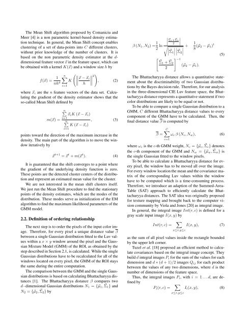
The Mean Shift algorithm proposed by Comaniciu and
Meer [4] is a non parametric kernel-based density estimation
technique. In general, the Mean Shift concept enables
clustering of a set of data-points into C different clusters,
without prior knowledge of the number of clusters. It is
based on the non parametric density estimator at the d-
dimensional feature vector ⃗x in the feature space, which can
be obtained with a kernel K(⃗x) and a window size h by
f(⃗x) = 1
nh d
n ∑
i=1
( ∥∥∥∥ ⃗x − ⃗x i
)
K ∥
h
∥2
, (2)
where ⃗x i are the n feature vectors of the data set. Calculating
the gradient of the density estimator shows that the
so-called Mean Shift defined by
m(⃗x) =
n∑
⃗x i K (⃗x − ⃗x i )
n∑
, (3)
K (⃗x − ⃗x i )
i=1
i=1
points toward the direction of the maximum increase in the
density. The main part of the algorithm is to move the window
iteratively by
⃗x t+1 = ⃗x t + m(⃗x t ). (4)
It is guaranteed that the shift converges to a point where
the gradient of the underlying density function is zero.
These points are the detected cluster centers of the distribution
and represent an estimated mean value for the cluster.
We are not interested in the mean shift clusters itself.
We just run the Mean Shift procedure to find the stationary
points of the density estimates, which are the modes of the
distribution. These modes serve as initialization of the EM
algorithm to find the maximum likelihood parameters of the
GMM model.
2.2. Definition of ordering relationship
The next step is to order the pixels of the input color image.
Therefore, for every pixel a unique distance value β
between a single Gaussian distribution fitted to the Luv values
within a x × y window around the pixel and the Gaussian
Mixture Model (GMM) of the ROI, as obtained by the
step described in Section 2.1, is calculated. While the single
Gaussian distributions have to be recalculated for all of the
windows located on every pixel, the GMM of the ROI stays
the same during the entire computation.
The comparison between the GMM and the single Gaussian
distributions is based on calculating Bhattacharyya distances
[1]. The Bhattacharyya distance β compares two
d - dimensional Gaussian distributions N 1 = {⃗µ 1 , Σ ⃗ 1 } and
N 2 = {⃗µ 2 , Σ ⃗ 2 } by
∣ ∣∣
β (N 1 , N 2 ) = 1 Σ1+ ⃗ Σ ⃗ 2
2 ln 2
∣
√ ∣∣∣ ∣ ∣ ∣ +
Σ1 ⃗ ∣∣ ∣∣ Σ2 ⃗ ∣∣
[ ⃗Σ1 + ⃗ Σ 2
2
] −1
(⃗µ 2 − ⃗µ 1 ).
1
8 (⃗µ 2 − ⃗µ 1 ) t
The Bhattacharyya distance allows a quantitative statement
about the discriminability of two Gaussian distributions
by the Bayes decision rule. Therefore, for our analysis
in the three-dimensional CIE Luv feature space, the Bhattacharyya
distance represents a quantitative statement if two
color distributions are likely to be equal or not.
To be able to compare a single Gaussian distribution to a
GMM, C different Bhattacharyya distance values to every
component of the GMM have to be calculated. Then, the
final distance value β is computed by
β =
(5)
C∑
ω c β (N c , N w ), (6)
c=1
where ω c is the c-th GMM weight, N c = {⃗µ c , Σ ⃗ c } denotes
the c-th component of the GMM and N w = {⃗µ w , Σ ⃗ w } is
the single Gaussian fitted to the window pixels.
To be able to calculate a Bhattacharyya distance for every
pixel, the window has to be moved all over the image.
For every window location the mean and the covariance matrix
of the corresponding Luv values within the window
have to be computed which is a time-consuming process.
Therefore, we introduce an adaption of the Summed-Area-
Table (SAT) approach to efficiently calculate the Bhattacharyya
distances. The SAT idea was originally proposed
for texture mapping and brought back to the computer vision
community by Viola and Jones [20] as integral image.
In general, the integral image Int(r, c) is defined for a
gray scale input image I(x, y) by
Int(r, c) =
∑
I(x, y), (7)
x≤r,y≤c
as the sum of all pixel values inside the rectangle bounded
by the upper left corner.
Tuzel et al. [18] proposed an efficient method to calculate
covariances based on the integral image concept. They
build d integral images P i for the sum of the values for each
dimension and d ∗ (d + 1)/2 images Q ij for each product
between the values of any two dimensions, where d is the
number of dimensions of the feature space.
Thus, the integral images P i , with i = 1 . . . d, are defined
by
P i (r, c) =
∑
I i (x, y), (8)
x≤r,y≤c