The Canadian Space Agency (CSA) Collision ... - SpaceOps 2012
The Canadian Space Agency (CSA) Collision ... - SpaceOps 2012
The Canadian Space Agency (CSA) Collision ... - SpaceOps 2012

Create successful ePaper yourself
Turn your PDF publications into a flip-book with our unique Google optimized e-Paper software.
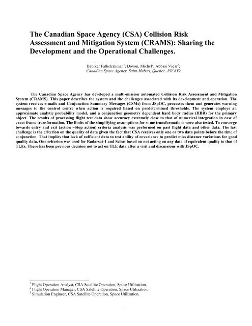
<strong>The</strong> <strong>Canadian</strong> <strong>Space</strong> <strong>Agency</strong> (<strong>CSA</strong>) <strong>Collision</strong> Risk<br />
Assessment and Mitigation System (CRAMS): Sharing the<br />
Development and the Operational Challenges.<br />
Babiker Fathelrahman 1 ; Doyon, Michel 2 ; Abbasi Viqar 3 ;<br />
<strong>Canadian</strong> <strong>Space</strong> <strong>Agency</strong>, Saint-Hubert, Quebec, J3Y 8Y9<br />
<strong>The</strong> <strong>Canadian</strong> <strong>Space</strong> <strong>Agency</strong> has developed a multi-mission automated <strong>Collision</strong> Risk Assessment and Mitigation<br />
System (CRAMS). This paper describes the system and the challenges associated with its development and operation. <strong>The</strong><br />
system receives e-mails and Conjunction Summary Messages (CSMs) from JSpOC, processes them and generates warning<br />
messages to the control centre when action is required based on predetermined thresholds. <strong>The</strong> system employs an<br />
approximate analytic probability model, and a conjunction geometry dependent hard body radius (HBR) for the primary<br />
object. <strong>The</strong> results of processing flight test data show accuracy extremely close to that of numerical integration in case of<br />
exact frame transformation. <strong>The</strong> limits of the simplifying assumptions for some transformations were also tested. To converge<br />
towards entry and exit (action –Stop action) criteria analysis was performed on past flight data and other data. <strong>The</strong> last<br />
challenge is the criterion on the quality of data given the fact that <strong>CSA</strong> receives only one or two data points before the time of<br />
conjunction. That implies that lack of sufficient data to test ability of covariance to predict miss distance variations for good<br />
quality data. One criterion was used for Radarsat-1 and Scisat based on not acting on any data of equivalent quality to that of<br />
TLEs. <strong>The</strong>re has been previous decision not to act on TLE data after a visit and discussions with JSpOC.<br />
1 Flight Operation Analyst, <strong>CSA</strong> Satellite Operation, <strong>Space</strong> Utilization.<br />
2 Flight Operation Manager, <strong>CSA</strong> Satellite Operation, <strong>Space</strong> Utilization.<br />
3 Simulation Engineer, <strong>CSA</strong> Satellite Operation, <strong>Space</strong> Utilization.<br />
1
I. INTRODUCTION<br />
<strong>CSA</strong> received its first warning of a close approach between Radarsat-1 and two space objects from JSpOC<br />
through NORAD in 2005. <strong>CSA</strong> and JSpOC have interactively done the planning and the verification of the<br />
avoidance maneuver . Only the miss distances were provided then. In 2009 <strong>CSA</strong> started receiving warning e-mails<br />
with miss distance and radial error. It had to estimate the in-track and cross track errors from the radial to construct<br />
a collision avoidance box. In 2010 <strong>CSA</strong> started to receive e-mails with miss distances and the errors in radial, intrack<br />
and cross track axes and finally the CSMs.<br />
In order to ensure that it is acting upon the best available information, <strong>CSA</strong> processes both the short-form<br />
email and the CSM. Due to satellite orbit information missing in the short-form emails, approximations are used to<br />
estimate the approach angle. Previously, <strong>CSA</strong> combined the error information for both satellites to construct a<br />
<strong>Collision</strong> Avoidance Box, and considered performing a collision avoidance maneuver if the situation was within the<br />
box. Since then, <strong>CSA</strong> has refined its methodology, implementing the Probability of <strong>Collision</strong> to get a more<br />
complete understanding of the risk involved in the close approach. Since the short-term email and the CSM have a<br />
well-defined format and structure, it was possible to automate the calculations. Thus, the CRAMS system<br />
automatically triggers as a result of incoming email and generates situational awareness data that is distributed to the<br />
appropriate operational teams almost instantly. <strong>The</strong> system is generic and robust enough to handle multiple<br />
missions that are operated at <strong>CSA</strong>, along with other missions, with no human intervention.<br />
II. CRAMS DESCRIPTION<br />
<strong>The</strong> CRAMS system has been operational since November 2011, supporting RADARSAT-1,<br />
RADARSAT-2 and SCISAT missions. Initially, the risk level was assessed primarily using the collision avoidance<br />
box. Since late 2011, the Probability of <strong>Collision</strong> calculations were incorporated into the system, along with a<br />
number of other improvements as a result of lessons learned. In <strong>2012</strong>, the MOST spacecraft (operated by the<br />
University of Toronto’s <strong>Space</strong> Flight Laboratory) was added to list of satellites for which <strong>CSA</strong> receives JSpOC<br />
notifications. CRAMS processes these notifications (CSM and short-form email) and distributes to the operational<br />
team at SFL. While MOST and SCISAT are not manoeuvrable spacecraft, an understanding of the threat to these<br />
satellites from space debris helps to understand the debris environment and plan mitigation strategies accordingly.<br />
In addition, if the close approach is with another operational satellite, avoidance operations could be coordinated<br />
with the other operators. Figure 1 shows the multi-mission operational context and interfaces of the CRAMS system.<br />
FIGURE 1. CRAMS BLOCK DIAGRAM<br />
2
A. CRAMS INPUTS AND OUTPUTS<br />
As shown in Figure 1, CRAMS processes JSpOC information and produces Threat Pre-Analysis data files,<br />
which include Risk Assessment data. Data is automatically emailed to a mission-specific distribution list. <strong>The</strong> data<br />
is compiled into a few formats: Excel spreadsheet, contains the original input data from JSpOC (email or CSM<br />
data), plus all the value-added content calculated in CRAMS, including graphics and charts. Summary text file,<br />
containing the most relevant information for operational decision-making from the original input data plus the valueadded<br />
content, (no charts).XML output file, contains the original input data from JSpOC (email or CSM data), plus<br />
all the value-added content, minus graphics and charts. And STK scenario files<br />
In current operations, only the Excel spreadsheet and summary text file are emailed to a mission-specific<br />
distribution list. <strong>The</strong> XML file and STK files stored on a network drive for review and analysis as necessary.<br />
Plugging the position and velocity information from JSpOC, along with the covariance data for both<br />
objects, into STK, CRAMS automatically builds the STK scenario and executes the STK-based conjunction<br />
analysis tools (STK/AdvCAT). This generates an STK conjunction analysis report containing data, plus<br />
visualization of the scenario. <strong>The</strong> visuals – both a 2D and 3D view - are automatically incorporated into the Excel<br />
file to provide a quick, intuitive understanding of the pending situation in space.<br />
3
III. CHALENGES<br />
A. SELECTION OF PROBABILITY MODEL AND REQUIRED FRAME TRANSFORMATIONS<br />
3.1.1Probability of <strong>Collision</strong><br />
3.1.1.1 Combined Covariance Matrix<br />
Initially the approach angle was used to combine the two sets of uvw errors in order to have a<br />
single, representative set of errors to construct a collision avoidance box. This was refined later using the<br />
combined covariance 1,2 . For probability calculations, this process must be extended to the full<br />
covariance matrix that is provided in the CSMs..<br />
Let the covariance matrices of the primary object and secondary object be C p and C s respectively each<br />
represented in their respective uvw coordinate systems, computed from the corresponding inertial position and<br />
velocity vectors. C r represents the combined covariance matrix expressed in the UVW frame of the primary object.<br />
To eliminate the errors associated with the transformations using the approach angle, a more precise<br />
transformation can be implemented. <strong>The</strong> state vector (position and velocity) of each objects (primary and secondary)<br />
is transformed into Earth Centered Inertial (ECI) coordinates. It is then used to define transformation matrices<br />
(direction cosine) from the primary and secondary frames and to transform the primary and secondary covariances<br />
in ECI coordinates. Subsequently, the relative position covariance (in ECI) is obtained by adding the two covariance<br />
matrices. Finally, the combined covariance matrix is converted back to the primary frame ( (u,v,w) of the primary).<br />
<strong>The</strong> approach is as follows. First, convert the R and V primary and secondary vectors from the EFG to the ECI<br />
frame (2 each, for a total of 4 transformations).<br />
, transformation matrices, T p and T s , can be created using , , , in the ECI frame such that<br />
(1)<br />
Where , , and , are the unit vectors of the primary spacecraft in the uvw frame defined by its ECI<br />
position vector. <strong>The</strong> vector is defined as a unit vector in the direction of the ECI object position vector from the<br />
center of the Earth to the spacecraft and calculated as follows:<br />
(2)<br />
<strong>The</strong> cross-track component,<br />
, is defined by the cross product of the ECI radial and velocity vectors:<br />
(3)<br />
4
And, finally, the in-track component completes the triad.<br />
(1)<br />
<strong>The</strong> transformation matrix for the secondary object is similarly constructed:<br />
(5)<br />
From that, the primary and secondary covariance matrices can be transformed into the ECI frame:<br />
(6)<br />
6<br />
(7)<br />
And the combined covariance for the encounter is the sum of the above two matrices.<br />
(8)<br />
Finally, C r in the UVW frame of the primary object is given by:<br />
C r = (9)<br />
3.1.2 PROBABILITY CACULATION<br />
While methods have been presented above to determine a level of severity to the spacecraft given limited<br />
information (such as DOI) when the full information of the JSpOC CSM is unavailable, a more thorough method of<br />
determining the severity of the event to the health and safety of the spacecraft is desirable. <strong>The</strong> metric that is most<br />
commonly used is the so-called “probability of collision”. Klinkrad 1 has provided a very thorough discussion of the<br />
measure of the probability of spacecraft collision and the descriptions below are based on [Ref.1 <strong>The</strong> more<br />
theoretical background can be obtained from [Ref.1 as well as Ref.2.<br />
<strong>The</strong> equation below represents the generalized expression of probability. It represents the integration of the<br />
probability density function over the volume. In its un-modified form, it is used for long encounter durations (i.e.<br />
minutes).<br />
(10)<br />
5
However, for short encounters, it can be reduced to a 2-D problem. This is based on the assumption of<br />
rectilinear motion in the encounter region. In this case, the probability value is independent of the error in the<br />
direction of the relative velocity vector.<br />
To simplify this equation, an encounter coordinate system (x,y,z) is defined at the time of closest approach<br />
(TCA) such that the origin is taken to be one of the two objects <strong>The</strong> x-axis is along the miss distance vector , the y-<br />
axis is along the relative velocity vector , and the z-axis along . <strong>The</strong> xz plane defines the encounter plane<br />
(also called the B-plane). In the encounter plane, the most significant contribution comes from the error component<br />
along the miss distance. Figure 2 2 shows the geometry of the encounter plane.<br />
z<br />
y<br />
V r<br />
(x e , 0, 0)<br />
R c<br />
secondary<br />
object<br />
Figure 2.<br />
primary<br />
object<br />
Encounter Plane Geometry<br />
x<br />
<strong>The</strong> equation below is the simplified, two-dimensional equation resulting from Equation 32 above. It is<br />
implemented in STK/CAT using two different approaches to approximate the double integral: a numerical one 3 and<br />
analytical ones. 2,4 (11)<br />
<strong>The</strong> above equation is not readily solvable, so a simplified solution is desired to allow for rapid processing<br />
independent of COTS software. <strong>The</strong> following sections describe two analytical methods to solve the twodimensional<br />
probability equation above.<br />
3.1.3 ENCOUNTER FRAME APPROACH<br />
<strong>The</strong> main assumption is that the variation of the probability density function is insignificant within the<br />
encounter region, i.e. a constant density. We have from Ref2.<br />
(12)<br />
In the above equation, r is the miss distance between the two objects.<br />
In order to implement (12), the following transformations are necessary for transforming the data in the<br />
form appropriate for use in the probability formula.<br />
6
In the encounter plane, the assumption of linear motion is valid for short encounters (duration of seconds)<br />
typical for LEO encounters. An encounter coordinate system is defined where the unit vectors are as follows. <strong>The</strong> x-<br />
axis is taken to be the miss distance vector as defined by:<br />
(13)<br />
<strong>The</strong> y-axis is taken as the direction of the relative velocity vector:<br />
(14)<br />
And the z-axis completes the triad:<br />
(2)<br />
From the above, the transformation matrix, to rotate the relative covariance matrix (where<br />
) in the primary frame to the relative position covariance matrix C in the encounter frame is as<br />
follows:<br />
(16)<br />
And the transformation of the covariance matrix is as follows:<br />
(17)<br />
Within the encounter coordinate frame, there is an “encounter plane” which is defined as the plane<br />
perpendicular to the velocity vector. Since the velocity vector is along the y-axis, this is therefore referred to as the<br />
“xz” plane.<br />
is a matrix that transforms the relative position covariance matrix r in the frame to the xz<br />
frame on the encounter plane to produce the 2-D covariance matrix . It is defined as follows:<br />
And the covariance matrix in the 2-D encounter plane is given by:<br />
(18)<br />
(19)<br />
where<br />
(20)<br />
7
Alternatively the above analysis can be extended as in Ref.1 and Ref.2 using the eigen values and eigen<br />
vectors to finally derive Eqs 21 and 22.<br />
(21)<br />
This has the approximate solution given by:<br />
(22)<br />
<strong>The</strong> approximate probability formula is known to follow closely the numerically computed probability in<br />
the ranges of operational interest as reported in Ref. 5.<br />
3.1.4 HARD BODY RADIUS<br />
As can be seen in Es 12 and(22 the probability result is directly proportional to the square Hard Body<br />
Radius (HBR) used. This makes the definition of this parameter a critical one in determining an accurate measure of<br />
the probability of collision.<br />
Typically, the cross-sectional size of the primary object is well known. For example, the effective hard<br />
body radius of RADARSAT-1 is either 7.5m or 2.0m depending on the side observed. If observed from the side<br />
(approach angle of 90º) the total length of the spacecraft is 15 m. If observed from the front (approach angle of<br />
180º), the total height of the spacecraft is 4 m.<br />
<strong>The</strong> following formula gives a close approach geometry dependent HBR for RADARSAT-1 and<br />
RADARSAT-2 (which have similar geometries).<br />
Where is the angle between the relative velocity vector ( ) and the -axis of the primary object. It is<br />
defined by:<br />
(23)<br />
(24)<br />
Where is defined in Eq. 4, and is the relative velocity vector.<br />
For SCISAT-1 a static HBR of 0.56 m is used, as its more compact nature lends itself more to an<br />
approximation of a sphere.<br />
For the secondary object, depending on the information provided by the CSM, the hard body radius will be<br />
based on the measured cross-section and referenced from the following table.<br />
Default values for the HBR of the secondary object are derived from the JSpOC CSM (small < 0.1 m 2 ,<br />
medium 0.1 m 2 < x < 1 m 2 , large > 1 m 2 ) and are inspired from ESOC’s approach to give a minimum HBR of 1 m to<br />
secondary objects. This is an open issue to be resolved considering the gravity gradient orientation of a lot space<br />
debris.<br />
8
Also, depending on the secondary object, additional information may be available from various sources.<br />
<strong>The</strong> combination of the hard body radius for the secondary object and the result of Equation (50) provides the value<br />
for R C in the probability equations.<br />
Historically, a safety factor of 50m around the objects was used when using a Box approach. This is no<br />
longer required when using probability and the dimensions of the objects (radius) are used (7.5m for RADARSAT-1<br />
and RADARSAT-2, 0.56m for SCISAT-1).<br />
B. VALIDATION OF PROBABILITY CALCULATION<br />
<strong>The</strong> implementation was compared with test cases evaluated by experts from 8 different organizations.<br />
<strong>The</strong>se results are summarized in Ref. 6and show good comparisons for a single event.<br />
In order to expand on the results from various comparisons with other systems computing probability have<br />
been conducted. <strong>The</strong> table below presents some of the results of a number of close approach events by comparing<br />
CRAMS with digitally computed probabilities .<br />
Event<br />
2011-09-07--R1-<br />
COSMOS_2251_DEB_csm201124826099<br />
2011-08-20--R2-<br />
DELTA_2_RB_csm201123024856<br />
2011-08-05--R2-<br />
COSMOS_2251_DEB_csm201121523811<br />
2011-08-05--R2-<br />
COSMOS_2251_DEB_csm201121423764<br />
2011-07-27--S1-CZ-<br />
4_DEB_csm201120523214<br />
2011-06-30--R2-<br />
COSMOS_2251_DEB_csm201118021655<br />
2011-06-21--R1-<br />
IRIDIUM_33_DEB_csm201117021052<br />
2011-06-15--R1-SL-<br />
3_RB_csm201116620764<br />
2011-05-25--R2-<br />
COSMOS_2251_DEB_csm201114319494<br />
Table 1. Probability<br />
Primary<br />
Object HBR<br />
(m)<br />
comparison results<br />
S<br />
econdar<br />
y Object<br />
HBR<br />
(<br />
m)<br />
2.1 1<br />
.0<br />
7.5 2<br />
.985<br />
7.5 1<br />
.0<br />
7.5 1<br />
.0<br />
0.55 1<br />
.0<br />
7.5 1<br />
.0<br />
2.1 1<br />
.0<br />
2.1 1<br />
.9<br />
7.5 1<br />
.0<br />
CRA<br />
MS<br />
Probability<br />
2.268<br />
E-05<br />
1.572<br />
5E-11<br />
3.273<br />
5E-10<br />
1.052<br />
1E-12<br />
5.929<br />
E-60<br />
2.661<br />
1E-05<br />
7.581<br />
E-03<br />
Pro<br />
babilitydigitalyl<br />
integ-1<br />
2.0<br />
55E-05<br />
0.0 1.0<br />
00E-30<br />
4.8<br />
07E-11<br />
6.4<br />
26E-10<br />
1.0<br />
78E-12<br />
1.0<br />
00E-30<br />
2.7<br />
07E-05<br />
0.0 1.0<br />
00E-30<br />
7.6<br />
95E-03<br />
P<br />
robabilitydigitally<br />
integ-2<br />
2.<br />
043E-05<br />
0<br />
0.<br />
4.<br />
769E-11<br />
6.<br />
353E-10<br />
1.<br />
070E-12<br />
1.<br />
189E-59<br />
2.<br />
690E-05<br />
0<br />
0.<br />
7.<br />
647E-03<br />
<strong>The</strong> above table shows that there is very good agreement between the probabilities as implemented in<br />
CRAMS and digitally integrated probabilities<br />
9
Table 2. CRAMS and digitally integrated Probabilities<br />
ase ID<br />
C STK<br />
(Alfano)<br />
1 4.1353e-<br />
005<br />
2 2.3544e-<br />
006<br />
3 9.8557e-<br />
006<br />
4 4.7409e-<br />
005<br />
5<br />
1.7301e-005<br />
6 4.1983e-<br />
005<br />
3e-005<br />
2e-019<br />
3e-005<br />
5e-005<br />
6e-005<br />
8e-005<br />
UVW ECI Orga<br />
nization1<br />
8.860 6.194 8.836<br />
3e-005 3e-005<br />
2.025 2.357 5.291<br />
7e-006 9e-007<br />
1.233 9.829 2.004<br />
8e-006 7e-006<br />
7.241 5.081 7.243<br />
7e-005 2e-005<br />
1.932 1.725 1.960<br />
2e-005 4e-005<br />
1.638 4.008<br />
2e-005 1.0869e-005<br />
App<br />
roach Angle<br />
119.5<br />
44.9<br />
71.0<br />
11.3<br />
71.1<br />
80.1<br />
As can be seen fromTables 1 and 2 there is good agreement between the CRAMS data sets and<br />
organization1 data. In particular the UVW data tracks very closely with other agencies results. It is likely that this is<br />
how they transform their covariance matrices for calculating probability. <strong>The</strong> ECI results are not significantly<br />
different from these other two sets of results, and they track very well with the STK results. Given that there are<br />
known approximations in the UVW approach and that the ECI transformation is a more rigorous method, the<br />
differences are not entirely unexpected. <strong>The</strong> overall correlation between the various data sets does lead to the<br />
conclusion that the CRAMS probabilities are being accurately calculated.<br />
C. IMPLEMENTATION<br />
Both the eigen and non-eigen methods for probability calculation have been implemented and lead to the<br />
same results.<br />
Following Eumetsat work, a weighted average of 3 values of probability evaluated at the centre, at +HBR/2<br />
and at –HBR/2 is also implemented.<br />
CRAMS will have the ability to calculate probability based on these alternate methods but the method based on Eq.<br />
12 will be used operationally as it is more robust.<br />
D. ENTRY AND EXIT CRITERIA<br />
A probability of collision greater or equal to 1.0e-04 represents the action criteria. This number has<br />
extensive operational heritage with other missions, including use by the <strong>Space</strong> Test Squadron (Air Force <strong>Space</strong><br />
Command <strong>Collision</strong> Avoidance process); it is also detailed in NASA’s Orbital Debris Conjunction Assessment and<br />
<strong>Collision</strong> Avoidance Strategy; and in Ref. 7 .<br />
A post-manoeuvre exit criterion is not nearly as well agreed upon and requires some measure of analysis.<br />
One method to determine the valid exit criterion would be to target a miss distance of at least to get out of<br />
the projected relative position covariance ellipse on the encounter plane which should drive the probability towards<br />
zero as elaborated in Ref. 8. However, the drawback of using this method is that it is not consistent with the methods<br />
of determining when to perform a manoeuvre in the first place (i.e. probability). In order to understand better the<br />
relationship between this threshold value and probability, a series of CSMs obtained from <strong>Space</strong>-Track.org was<br />
processed to determine the approximate probability of collision for each event. Only events that had a probability of<br />
greater than 1E-04 are presented here. Additionally, for each event, the value was determined as the final<br />
miss distance, and the probability calculated from that. Both the initial probability (red squares) and the threshold<br />
probability (blue diamonds) are plotted below for each event.<br />
As can be seen, the threshold probability associated with<br />
8 is not constant from event to event.<br />
This is likely due to the fact that the covariances are not constant, but vary from event to event as well. <strong>The</strong>re is a<br />
10
trend towards numbers generally below 1E-05 with the lowest two between 1E-11 and 1E-13 . If one looks,<br />
however, at where most of the “Exit” data is plotted, one can see that the data generally is above 1E-09. From this<br />
plot it would be reasonable to use 1E-09 as the exit criteria for burn planning based on the threshold. In<br />
addition, 1E-09 is referenced in Ref. 7as the criterion for a successfully sized manoeuvre.<br />
Figure III-1 Exit criteria based on encounTer plane geometry<br />
Also plotted, are green triangles which show the approximate probability for three actual escape<br />
manoeuvres performed for this data set. Of these three events, one burn would not have exceeded the “exit criteria”.<br />
In fact, that one burn (the first of the three in the above plot) was not even large enough to create a < 1E-04<br />
probability of collision. However, the other two were large enough that if the value were used as a<br />
criterion, the burns would have been large enough to pass this criterion. One would have achieved a 1E-08<br />
probability, and the other ~1e-22.<br />
It is clear that the previous method of sizing burns (escape from a collision avoidance box created based on<br />
location errors) is not consistent with a probability-based exit criterion. This does not specifically cast doubt on<br />
either method, but it does show that there is no one “correct” method for determining when a situation is “safe”. <strong>The</strong><br />
goal here in choosing a probability exit criterion is to maintain consistency in how one defines a high and low risk<br />
situation.<br />
E. IMPACT OF MANOEUVRE ON COVARIANCE MATRIX<br />
Once it has been decided that the probability of collision is high enough that an escape manoeuvre is<br />
warranted, the effect on the probability of collision by the new displacement as well as by the error induced by<br />
uncertainty in the burn must be considered.<br />
<strong>The</strong> new location of the spacecraft at TCA can be determined via the CW equations 9 , and the new miss<br />
distance can be evaluated as in Ref. 10 .<br />
If it were the case that the requested manoeuvre size had zero error with respect to the actual delivered<br />
change in velocity, the probability can be calculated with the original covariances and the new close approach<br />
vector. This assumes that the original covariances are constant over the region of space that includes the original<br />
close approach location and the new time of closest approach. However, the manoeuvre itself carries with it some<br />
uncertainty, so that must be factored into the probability.<br />
We make use of the assumptions above, that the covariances of the locations of the two objects are not<br />
changed due to the change in location and the change in the time of closest approach. Additionally, it is assumed<br />
that the error in the change in velocity is an independent source of error. <strong>The</strong>refore, the final covariance of the<br />
primary object (the one assumed to be manoeuvring) is simply a summation of the original covariance and the error<br />
in the change in velocity.<br />
Indicating that the error in the change in velocity is directly proportional to the error in the final in-track<br />
location as the change in velocity is to the change location.<br />
In a routine RADARSAT-1 manoeuvre, the worst case observed error for an in-track manoeuvre, ε m , is 5%<br />
of the change in velocity. (In actuality, the error observed is the error in the change in semi-major axis of the<br />
manoeuvre, but this is proportional to the change in velocity 7 .<br />
11
Substituting the sigma value of 5% (R1 maximum error in the worst case, i.e. 3 sigma error) we have:<br />
(Refs. 7,9) (25)<br />
<strong>The</strong> covariance is then simply added to the initial covariance of the primary object at the time of closest<br />
approach to arrive at a new, burn-induced covariance. <strong>The</strong> probability is calculated as in the pre-burn case but with<br />
the new post-manoeuvre covariance. Note that the values for the covariances due to the manoeuvre in the radial and<br />
cross-track are assumed to be zero.<br />
It should be noted that an in-track change in velocity does induce a radial change in the location of the<br />
satellite along the orbit. Specifically, for a single thrust at a single point in the orbit, the radial position will be<br />
changed such that it is maximized at the opposite side of the orbit as the manoeuvre and minimized (actually is 0) at<br />
the point in the orbit that the manoeuvre occurs. However, these changes in radial position are small and are constant<br />
unlike the changes in the in-track position which are significant larger and build up over time. For the purposes of<br />
this analysis they are ignored.<br />
G. DATA QUALITY Indicators<br />
3.7.1 TLE QUALITY AS THE LIMIT FOR SP DATA QUALITY<br />
<strong>The</strong> level of measurement errors, the level of orbit prediction and determination errors in the data received<br />
from JSpOC may lead to erroneous or misleading results when computing probability or D Prior to the advent of the<br />
JSpOC notification system currently in place, the only method of determining whether close approach events were<br />
to occur was by comparing the widely available TLEs that are disseminated for the known objects in low-Earth<br />
orbit. However, it has since become evident that the errors on these vectors are much too large to effectively<br />
generate believable close approach events.<br />
At the CSM workshop in October 2010 (, estimates for TLE prediction were presented for 18 and 72 hours<br />
prediction cases 11 . In the case of <strong>CSA</strong> spacecrafts (LEO altitude > 500km),<br />
In order to determine the impact of these values on the previous analyses, the below plot is presented. It<br />
shows the In-track 1-sigma error from a series of 60+ CSMs, with the blue line. Superimposed on this line, are<br />
orange diamond markers which indicate which of these events had resulting probabilities of greater than 1E-04, the<br />
previously proposed threshold for determining whether an event requires an escape manoeuvre. (<strong>The</strong>y are, in this<br />
case, simply Boolean markers; they do not represent a value on a scale.) Finally, the red line represents the above 72<br />
hours TLE prediction error. (<strong>The</strong> assumption is that the majority is in the in-track direction for this plot, when in<br />
reality it is RSS.<br />
Figure III-2 In-track Errors compared to TLE ERROR Limits<br />
<strong>The</strong> primary information to take away from this plot is that there are several events (7 in the above<br />
sampling) that would be defined as requiring a manoeuvre, but with in-track errors that exceed the known magnitude<br />
for TLE errors. For this reason, it is recommended here that a limit on the magnitude of measured errors by JSpOC<br />
12
e imposed prior to deciding on whether to perform a manoeuvre. This limit would be the limit of TLE RSS errors,<br />
propagated to 72 hours, and would be imposed on both primary and secondary objects. If either of the two objects<br />
were to violate the limit of 1.7km, no decision would be made until the errors were reduced to a lower level.<br />
3.7.2 CSM QUALITY INDICATORS<br />
CSM Data: these are: how recent the data are, the data arc with respect to the optimum arc,<br />
and the number of data points used in orbit determination are OD quality indicators available in the CSM.<br />
3.7.3 DATA CONSISTENCY<br />
When you have more than one CSM the ability of the previous covariance to predict the recent one gives a<br />
measure of data consistency. But if there only one covariance before the close approach then that measure is lacking<br />
and the use of a cut-ff limit on RSS error of the SP data as the TLE is a reasonable alternative.<br />
H. TIMELY PRODUCTION OF A MANEUVER TRADE SPACE<br />
In the situation where a close approach alert leads to a manoeuvre, a manoeuvre trade space is required to<br />
provide options within the close approach and system constraints that enables the selection of the optimum<br />
avoidance manoeuvre for increasing the separation distance and reducing the risk of collision to an acceptable level<br />
(e.g. 5 orders of magnitudes lower than 1.0e-04). Software such as STK Astrogator and CAT allow computing a<br />
manoeuvre trade space based on the information provided by the CSM information. Such calculation is computer<br />
intensive and requires the use of expensive software. McKinley 10 presents a simplified method allowing fast<br />
calculation of sufficient level of accuracy following an analytic approach rather than the numeric approach<br />
employed in an older version of CRAMS using STK Astrogator and CAT and tools similar to it. This analytic<br />
approach has been implemented in-house and tested.CRAMS produces a number of maneuver trade space charts. In<br />
addition to the charts, the data is also available in table form.<br />
.<br />
ACKNOWLEDGMENTS<br />
In the writing of this paper and the development of the associated operational tools, we would like to<br />
acknowledge the feedback and information provided by various space agencies and satellite operators. <strong>The</strong>ir<br />
feedback was instrumental in allowing us to develop our expertise in a short period of time. Namely, we would like<br />
to recognize ESA-ESOC, EUMETSAT, CNES, AFSPC and the Joint <strong>Space</strong> Operations Command (JSpOC).<br />
REFERENCES<br />
1<br />
Klinkrad, Heiner, <strong>Space</strong> Debris Models and Risk Analysis, PARAXIS PUBLISHING Ltd, Chucgdster,UK, 2006,<br />
chap 8<br />
2<br />
Chan, Kenneth, <strong>Space</strong>craft <strong>Collision</strong> Probability, <strong>The</strong> Aerospace Press, El Segundo , California, 2008,<br />
chap 1-6.,2008<br />
3<br />
Alfano, Salvatore A Numerical Implementation of Spherical Object <strong>Collision</strong> Probability,<br />
<strong>The</strong> Journal of Astronautical Sciences - Jan – Mar 2005<br />
4 Patera, R. P. General Method for Calculating Satellite <strong>Collision</strong> Probability, AIAA Journal of Guidance,<br />
Control, and Dynamics Vol 24, No 4. July – August, 2001<br />
13
5 Alfriend, K. et al. Probability of <strong>Collision</strong> Error Analysis - 1999<br />
6 Wysack, Joshua, et al. <strong>The</strong> JAXA report (<strong>Agency</strong> probability comparison methods) -<br />
2010, 2011<br />
7<br />
Righetti, Pier Luigi et al. Handling of conjunction warnings in Eumetsat Flight Dynamics - -<br />
8 Frigm, Ryan C. et al. Assessment , Planning & Execution considerations<br />
for Conjunction Risk Assessment and Mitigation Operations, <strong>Space</strong>Ops 2010 - 2010<br />
9 Cliff, Eugene M. Clohessey-Wiltshire Analysis Oct 23, 1998<br />
10 McKinley, David Manoeuvre Planning for Conjunction Risk Mitigation with Ground Track Control Requirements<br />
11<br />
Kaya, Denise & Ericson, Nancy JSpOC/ESA post conjunction event analysis - Oct 2010<br />
- -<br />
14