optimisation of a fast monohull with cfd-methods - TUHH

10 th International Conference on Fast Sea Transportation
FAST 2009, Athens, Greece, October 2009
OPTIMISATION OF A FAST MONOHULL WITH CFD-METHODS
Tobias Haack 1 , Stefan Krüger 2 , Hendrik Vorhölter 2
1 Product Development, Flensburger Schiffbau-Gesellschaft mhH & Co KG (FSG), Batteriestrasse 52, 24939
Flensburg, Germany
2 Institute of Ship Design and Ship Safety, Hamburg University of Technology (TUHH), Schwarzenbergstraße
95C, 21073 Hamburg, Germany
ABSTRACT
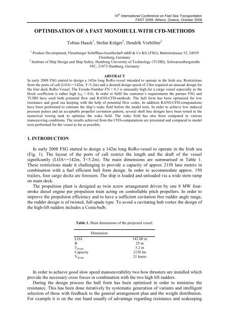
In early 2008 FSG started to design a 142m long RoRo-vessel intended to operate in the Irish sea. Restrictions
from the ports of call (LOA

ehaviour to design the vessel with the longitudinal centre of gravity significantly aft of the
main frame. On the other hand an exaggeration leads to blunt aft bodies. Therefore the decks
house has been placed at the bow.
Because of the relatively high block coefficient it was essential to focus on the wave
making resistance as well as on the wake field. A bad wake field does not only influence the
comfort level in means of noise and vibrations but indirectly the propeller efficiency leading
to higher fuel consumption. Therefore a number of appendage arrangements have been
analysed using RANS-methods. The most promising variants have been tested in the towing
tank including wake field measurements. For the integration of RANS-methods in the design
process a new process chain has been implemented.
Fig. 1. Sideview of the projected vessel.
2. HULL FORM DESIGN WITH POTENTIAL FLOW METHODS
Based on FSG's specific numerical and experimental experience with RoRo-vessels, the
hullform was optimised for a speed range from 19 to 22.5 knots for the design draught of
5.20m. Furthermore lower speeds and lighter loading conditions were considered during the
hullform design process. Several different hullform alternatives were evaluated, varying
· length, volume and shape of the bulbous bow
· position of forward and rearward shoulder
· bilge radius
· shape and arrangement of aftbody tunnels
· transom shape, immersion and buttock slope of the aftbody
· location of knuckle lines according to the streamlines of the flow.
Care was taken for both a minimum of wave resistance (expressed by the generated wave
pattern) as well as harmonic pressure gradients. Besides, the wetted surface was kept as small
as possible. FSG uses the non-linear potential flow panel method KELVIN (Söding 1999) for
predicting the wave resistance, taking into account dynamic sinkage and trim. The results are
presented as plot of wave contour and pressure distribution. KELVIN is integrated in FSG’s
ship design system E4 (Bühr et al. 1988) as part of the implemented process chain from hull
form geometry definition over grid generation to CFD and post-processing.
The results of the CFD computations show the low wave making of FSG's design for both
the transverse and the diverging wave systems. This leads to a very low wave making
resistance and consequently to low wake wash. Minimising transverse waves reduces the
wave resistance significantly, although transverse waves are difficult to observe in the towing
tank.
Details of the hull form design and optimisation are briefly described in the following
sections.

2.1 Length, volume and shape of the bulbous bow
FSG's concept for bulbous bow design is that the bulb should generate an extreme lowpressure
zone located on the bulbous bow top. This low pressure zone (which generates a
significant wave through) reduces the height of the bow wave. Whether a specific bulbous
bow design will generate a low pressure region depends mainly on the vessel's speed, length
and volume of the bulbous bow. To support the downward flow of the streamlines, the
inflection points of the inner buttocks are located exactly in the stream lines. Fig. 2 shows the
pressure distribution of the present bulbous bow design. For ballast conditions, the bulb was
designed such that it will act as a sharp elongated waterline.
Fig. 2. Pressure distribution at bulbous bow.
2.2 Forebody: Interference of wave system
The position of the shoulder was selected for optimum interference between bowgenerated
and shoulder-generated wave patterns. As the bow-wave is influenced strongly by
the stem shape and the bulbous bow design, the position of the shoulders has to be selected
individually for each specific design.
Fig. 3 illustrates the good interference of bow- and forward shoulder generated waves: the
diverging wave pattern generated by the forebody in the resulting wake is very small. Besides,
the pressure gradient is harmonised, so viscous resistance is reduced due to a harmonic flow.
Fig. 3. Wave pattern at 21knots.
2.3 Aftbody: Stern tunnels, transom shape and immersion
Several alternatives of aftbodies were analysed. Important factors besides minimum wave
resistance were: low propeller induced pressure fluctuations on the hull, a harmonic wake
field for the propeller and intact as well as damage stability requirements.

For typical RoRo and RoPax hull designs a large share of the wave resistance is generated
by the transverse stern waves. While in model tests and ship operation stern waves are a lot
more difficult to target than the visually more pronounced longitudinal wave systems, CFD
analysis allows for a good insight and thus optimisation of this important part of wave making
and resistance.
The aftbody design features a twin tunnel arrangement, which allows increased tipclearance
above the propeller and thus low propeller induced pressure fluctuations. The slope
of the aftbody buttocks was optimised with focus on harmonic pressure gradients in order to
avoid flow separation and allow for a harmonic wake field as well as minimum resulting stern
waves.
2.4 Model test results
To verify the power prognosis and to compare the various appendage design variants,
model tests have been performed at the Hamburg Ship Model Basin (HSVA).
The results demonstrate that the target to design a vessel with low fuel consumption in
combination with an acceptable wake field has been reached. Fig. 4 shows the wave pattern
under design conditions which is comparable to the computational results. In order to get an
impression of the hydrodynamic quality of the hullform design, the power demand has been
compared to similar vessels by HSVA (see Fig. 5). Three designs in HSVA’s database have
been identified to have nearly the same ship lengths and block coefficients. For the purpose of
comparison the power demand has been adapted to the displacement of FSG’s design. The
diagram clearly shows that FSG’s hull form design leads to a significantly lower power
demand (approx. 20%) than all comparable vessels in the database especially in the speed
range 20 to 23 knots. Considering actual fuel prices this results in a reduction of operational
costs of 1.5-2 Million US-$ per year.
The results of the wake field measurements are described in chapter 3.3.
Fig.4. Photo from model test at 21knots.
Fig. 5. Comparison of power demand.

3. APPENDAGE DESIGN WITH RANS-CFD METHODS
The appendages, namely shaft line, bossing and brackets, are analysed with the help of
RANS-CFD methods. In the following the motivation for RANS-CFD analysis is described,
followed by a short description of the RANS-CFD process used at the Institute of Ship Design
and Ship Safety (SSI). The section continues with an investigation of the initial and an
improved appendage design and concludes with a comparison of the two CFD-codes Comet
(ICCM 2001) and FreSCo (Marci 2009).
3.1 Motivation for the RANS-CFD Analysis
The aspect of vibrations is a crucial point in most modern designs of RoRo-ferries. The
main source for vibrations on board ships is the propeller as it is working with an
inhomogeneous inflow. Especially in the area of the twelve o’clock position the inflow speed
is decreased significantly which leads to higher angles of attack for the propeller blades. This
ends in higher loads on the propeller and the ship’s hull. Concerning twin-screw-vessels the
disturbances of the propeller inflow are mainly generated by the shaft line, bossing and
brackets and not by the hull form itself. This has to be considered for the design of the shaft
line in addition to the requirements of mechanical strength and functionality. The shaft
bossing and the brackets have to be aligned properly to avoid unnecessary disturbances of the
propeller inflow.
The fluid flow around a bare hull is mainly driven by potential flow effects. Therefore, the
overall hull design can be efficiently and accurately analysed and optimised with potential
flow methods. For the analysis of the wake field viscous flow effects like the development of
the viscous boundary layer and vortices become more important. Thus, RANS-CFD-methods
have to be used for the analysis of a flow field around the appendages.
For the optimisation process the quality of the wake field has to be quantified. A wake
field of a good quality should lead to low pressure pulses. Thus, one method for the quality
analysis is the measurement of pressure pulses in the cavitation tunnel. These investigations
are performed for every project at FSG in later design stage. But, the cavitation tunnel tests
require a physical model and are therefore not very useful in the early design stage. Another
method is the numerical estimation of the pressure pulses. The inhomogeneous wake field is
used as input for a propeller computation. This of course requires an available propeller
design and the wake field has to be determined. A cruder but faster method, which can be
used in the early design process, is the use of a wake field quality criterion. Several criteria
exist. Most of them are based on an averaging of the variation of the axial inflow velocity.
The criterion used in the present work was developed by Fahrbach and Krüger (see Fahrbach
2004) and is based on the velocity gradient and the variation of the angle of attack on a single
propeller blade during one turn. Thus, not only the axial but also the tangential velocity
component is used, which is an advantage compared to simpler models.
3.2 RANS-CFD process
In order to use RANS-CFD methods in the initial design process a fast and robust CFDprocess
chain is required. The RANS-CFD process used at SSI consists of the ship design
system E4 and the finite volume mesh generator HEXPRESS (NUMECA 2008) for the preprocessing.
For the processing two different RANS-codes are used. On the one hand Comet,
which is a well validated tool for marine purposes, and on the other hand FreSCo, which is an
in-house development of the Institute of Fluid Dynamics and Ship Theory at TUHH, HSVA
and the Maritime Research Institute Netherlands (MARIN). The post processing, i.e. data
visualisation, is done with ParaView (Squillacote 2008).
The described RANS-CFD process allows the analysis of a ship model including
appendages within a few hours starting from the CAD-geometry in E4 including the
preparation of the geometry, set-up of the computational model, processing and postprocessing.
The computations are usually performed in model scale in order to speed up the

processing on the one hand and on the other hand to allow a direct comparison of the results
to model measurements. In order to reduce the computational effort the free surface is not
modelled in the RANS-computations. Either the free surface is taken from the KELVIN
computation and included in the geometry description 1 or the computation is performed with a
double body model with symmetry planes. All computations in this section are done with a
fixed free surface from the KELVIN computation in combination with the RANS-solver
Comet. The finite volume mesh has about 500,000 cells. The thickness of the first cell layer
on the hull surface is derived from a desired y+ between 60 and 100. The mesh generation and
the computation are performed on a standard PC with 12GB RAM and two quad core
2.33GHz CPUs.
Several designs of shaft line and shaft line bossings were investigated. The results of two
of them are presented in the following sections. The first design (variant 1) is the first
appendage design, which was tested in the towing tank for this project. The second one
(variant 2) is one of the variations developed from the first one using the information gained
from the CFD-results. All variants were tested by CFD, but only variant 1 and 2 were tested
in the model basin.
3.3 Investigation of the initial design
In the first step the results of the RANS-CFD computation are compared to the model test.
As the CFD-computations are performed including a free surface from a potential flow code,
a difference between the computed and measured resistance has to be expected. But it came
out that the difference between the measured and computed resistance is less than 1%. The
two wake fields are shown in Fig. 6. All wake fields presented are for the port side of the
vessel and seen from the aft. The contours indicate the axial velocity whereas the arrows
indicate the velocity in the propeller plane.
Fig. 6. Measured (left) and computed (right) wake field for bossing design variant 1.
It can be seen that the qualitative and quantitative coincidence between the results is very
good, although the shaft brackets, which are of course present in the model tests, are not
modelled in this first computation. The major difference can be seen in the thickness of the
boundary layer, which is thicker in the computation. This is an effect which can often be
observed in CFD-computations and is an object of further investigations. Another difference
is the flow shadow of the shaft line at the one o’clock position, which is more pronounced in
the CFD result than in the measurement. The coincidence is also shown by the analysis of the
wake field which is presented in Table 2. The mean velocities are normalised by the model
speed and the differences with the results from the model test. One can see that the wake field
1 In this case the floating condition is also taken from the potential flow computation.

quality is captured very well as the differences are less than 1%. The large relative difference
in the nominal wake fraction can be explained by the large zone of deceleration at the eleven
o’clock position, which is not so pronounced in the CFD result. Furthermore the wake number
is small which makes it more difficult to capture it correctly 2 . This is also the case for the
vertical velocity component. 3
Table 2. Analysis of measured (Exp) and computed (CFD) wake fields of design variant 1 and 2. The
differences are normalised with the values from the experiments and given in %.
Exp1 CFD1 Difference Exp2 CFD2 Difference Difference
Variant
CFD1-Exp1
CFD2-Exp2 Exp2-Exp1
Radial quality factor 0,9801 0,9831 0,31 0,9824 0,9799 -0,26 0,24
Circumferential quality factor 0,7243 0,7200 -0,59 0,7464 0,7475 0,16 3,05
Wake field quality factor 0,7098 0,7078 -0,28 0,7332 0,7325 -0,10 3,30
Nominal wake fraction axial 0,0812 0,0979 20,65 0,0836 0,0896 7,19 2,97
Nominal wake fraction total 0,0810 0,0978 20,76 0,0835 0,0895 7,26 3,00
Mean cross flow -0,0564 -0,0548 -2,87 -0,0566 -0,0525 -7,21 0,23
Mean up flow 0,0565 0,0690 22,06 0,0535 0,0708 32,19 -5,31
The designers develop an improved appendage design by using the pressure distribution on
the surface of the shaft line and shaft bossing together with section plots of the velocity field.
Fig. 7 shows the pressure distribution on the appendages for the first design. The pressure is
normalised with the stagnation pressure. The left side shows the inner and the right side the
outer side of the shaft bossing. The relatively large areas of low-pressure (red colour) indicate
that the bossing is not properly aligned in the fluid flow. This can also be seen in Fig. 8 where
a section close to the end of the shaft bossing is shown.
Fig. 7. Pressure distribution on the inside (left) and outside (right) of the shaft line, design variant 1.
Fig. 8. Section plot of the velocity field in the area of the stern tube bossing.
2 The difference of the mean nominal inflow speed is less than 2%.
3 The vertical velocity component is also affected by the trim which is not necessarily the same for the
measurement and the computation.

3.4 Investigation of the improved design
With the information gained in the first computations the geometry of the shaft line
bossing is modified and aligned to the direction of the fluid flow. The computed pressure
distribution (see Fig. 9) is more harmonic than for the first variant. There are less The
comparison of the wake fields shows the area of decreased velocity at the twelve o'clock
position could be reduced. The peak value of the normalised axial velocity is increased from
0.40 to 0.42. The wake field quality factor is increased from 0.708 to 0.733 which is an
improvement of 3.3%. Experiences from other projects at FSG and TUHH show, that this
increase of the wake field quality already reduces the risk of harmful cavitation and the level
of pressure pulses significantly.
Fig. 9. Pressure distribution on the inside (left) and outside (right) of the shaft line, design variant 2.
The optimised appendage design was tested in the towing tank. The measured wake field is
shown in Fig. 10 on the left side. The coincidence between the measured and the computed
wake field is acceptable as it was for the first case. Differences can be seen mainly at the
formation of the vortices above the shaft line. But this is on the inner radii which are of minor
interest concerning the pressure pulses. The resistance was slightly reduced. However, the
propulsion test show that the shaft power needed for the design speed remains the same. This
is a positive result, as the wake field quality is improved without negative effects on the total
propulsion efficiency. The velocity field upstream of the propeller is used to align the shaft
brackets.
Fig. 10. Measured (left) and computed (right) wake field for improved bossing design variant 2.
3.5 Comparison of the two RANS-CFD codes
For the improved appendage design computations are performed with the two RANS-
CFD-codes Comet and FreSCo. Fig. 11 shows the comparison of the computed wake fields.
The computations are performed on the same mesh with the same settings as far as this is

possible. The turbulence modelling differs between FreSCo and Comet. Thus, one can not
expect identical results. Nevertheless one can see in Fig. 11 that the resulting wake fields for
the two codes are nearly identical. The characteristics of the wake field are reproduced better
in the FreSCo computation although the velocity minimum in the twelve o’clock region is not
reproduced correctly as well. The difference in smoothness of the contour lines between the
Comet and the FreSCo result, is a result of different interpolation schemes in the postprocessing.
Fig. 11. Comet (left) and FreSCo (right) result for the improved bossing design variant.
4. WAKE FIELD INVESTIGATION FOR THE MANOEUVRING VESSEL
For Ro-Ro-vessels operating in short sea services not only the straight ahead condition but
manoeuvring conditions are of concern for a design improvement. This should also be
considered for the appendage design. Therefore, computations of the wake field for the
manoeuvring vessel are performed. In the following section the set up of the RANS-CFD
computations for these computations is described. This is followed by a short view on the
achieved results.
4.1 Set-up of the computations
The geometry is the same as for the computations with the improved design. Despite the
fact that the shaft brackets are included in the model. This is done, because it is expected that
in drift motion the brackets will cause more disturbances in the fluid flow as in the straight
ahead motion. For the straight ahead condition, especially for twin-screw vessels it is
adequate to assume that the fluid flow around the ship’s hull is symmetric. For the
manoeuvring conditions this is of course not valid. Thus, both sides of the hull have to be
concerned. The computations are performed without change of heel and trim. Thus, the
influence of the free surface on the wake field is still considered to be small and the free
surface is modelled as flat plane.
Computation are performed for 15 different manoeuvring conditions. Pure drift conditions
are analysed with 6 different drift angles β = 0°, -2.5°, -5°, -10°, -15° and -20° as well as
combined drift and yaw motions with full scale turnings rates of -100°/min, -75°/min and -
50°/min and drift angles β of 0°, -10° and -20°. The range of drift angles and turning rates are
chosen after an analysis of manoeuvring simulations for the full scale vessel.
4.2 Data analysis and results
For the analysis of the nominal wake fields the fluid flow is read out on discreet vertices in
the propeller plane. These read out points are located on concentrical circles centred on the
shaft line with a radius varying from 0.3 to 1.2 in steps of 0.1 of the half propeller diameter.

In Fig. 12 the normalised velocity in the propeller plane is shown. The left figure indicates the
cross flow and the right one the axial flow. The abscissa is the body velocity of the vessel in
the propeller plane v ' :
v'
= (sin( β ) ⋅U
− xP ⋅r)
/ U
(1)
U is the track speed, β the drift angle, x
P
x-coordinate of the propeller plane relative to
the centre of rotation and r the turning rate. For each propeller side and each turning rate one
curve is shown. The port side propeller (PS) is the outer and the starboard side propeller (SB)
the inner propeller. One can see that the mean horizontal velocity in the free stream on the
port side is only depending on the body motion. Whereas on the inner propeller it makes a
difference whether the vessel is in pure drift or in a combined drift and yaw motion.
Fig. 12. Analysis of the nominal cross flow (left) and axial (right) wake field velocities.
This becomes more obvious if the velocity plots in Fig. 13 to 15 are compared. The figures
show section plots of the velocity field in the propeller plane. The white grid shows the read
out points for the wake field. Fig. 13 shows the straight ahead condition. The fluid flow is not
fully symmetrical. This is caused by transient effects in the computation. The influence of the
shaft brackets is captured very well compared to the measurement (see also Fig.10). The
horizontal body motion in propeller plane is nearly identical in the second and third case
v ' = −0.1028 and v ' = −0. 0979 respectively. But the flow field is different especially
concerning the vortex structures at the skeg.

Fig. 13. Velocity field in the propeller plane with 0° drift angle and 0°/min turning rate.
Fig. 14. Velocity field in the propeller plane with 15° drift angle and 0°/min turning rate.
Fig. 15. Velocity field in the propeller plane with 10° drift angle and 50°/min turning rate.

5. CONCLUSIONS
In this paper a new FSG RoRo-ship design has been introduced with focus on power
demand and wake field. As the ship dimensions are limited it was challenging to design a
vessel with low fuel consumption at relatively high Froude numbers combined with a high
block coefficient. An additional challenging demand was to design the aftbody and the
appendages in such a way that the wake field quality makes it possible to design an efficient
propeller causing low noise and vibration levels.
The hull form has been optimised using potential flow methods in order to minimise the
resistance and consequently the propulsion power. Parallel to the resistance optimisation
process, RANS-computations have been done to analyse the wake field. Various aftbody
designs including different appendage configurations have been analysed using viscous flow
simulations. The quality of the resulting wake fields has been analysed using wake field
quality factors. The results of the computations have been compared to model test data.
The results clearly show, that combining FSG’s standard optimisation process using
potential flow methods with RANS-CFD for the optimisation of the wake field leads to good
predictions of the wave pattern and the wake field. The advantages of each of the both
methods have been taken: the fast and robust potential flow method enables the designer to
optimise the hull form efficiently while the more costly viscous flow computations give a
better inside into the flow details where necessary.
For the ship design described in this paper a significant power saving has been achieved
(approx. 20%) compared to similar vessels as shown by the data from the model basin. This
fact clearly indicates the potential of the optimisation process using boundary element
methods.
The appendages have been designed using RANS-Methods. The described method delivers
computed wake fields with sufficient accuracy for practical ship- and basic propeller design.
Not only the design condition but manoeuvring conditions have been considered for the wake
field computations as well. The results of these computations will be used for further propeller
performance investigations and manoeuvring simulations.
REFERENCES
Bühr, W., Keil, H., Krüger, S. (1988). Rechnereinsatz im Projekt. Jahrbuch der Schiffbau Technischen
Gesellschaft 82. p 352 et seqq. Springer-Verlag. Berlin. 1989 (in German)
ICCM (2001). Comet, Version 2.00, User Manual. Institute of Computational Continuum Mechanics. Hamburg,
Germany
Fahrbach, M. (2004). Bewertung der Güte von Nachstromfeldern. Diploma thesis. Hamburg University of
Technology, Hamburg, Germany (in German).
Marci, J. (2009). Introducing FreSCO. The New RANS Solver for Maritime Applications. News Wave of
Hamburg Ship Model Basin. Hamburg, Germany. 2009
NUMECA (2007). User Manual, Hexpress v2.5. Brussels. Belgium.
Söding, H. (1999). Das Wellenwiderstands-Programmsystem KELVIN. IfS Report. Universität Hamburg.
Institut für Schiffbau. Hamburg, Germany (in German).
Squillacote, Amy (2008). The ParaView Guide. 3 rd edition. Kitware Inc.
Vorhoelter, H. & Krueger, S. (2007). Optimization of Appendages Using RANS-CFD-Methods. Proceedings
10 th Numerical Towing Tank Symposium, Hamburg, Germany.