Stochastic Modelling Solutions to Exercises on Time Series∗

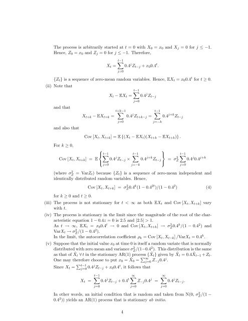
The process is arbitrarily started at t = 0 with X 0 = x 0 and X j = 0 for j ≤ −1.
Hence, Z 0 = x 0 and Z j = 0 for j ≤ −1. Therefore,
∑t−1
X t = 0.4 j Z t−j + x 0 0.4 t .
j=0
{Z t } is a sequence of zero-mean random variables. Hence, EX t = x 0 0.4 t for t ≥ 0.
(ii) Note that
and that
and also that
X t+k − EX t+k =
∑t−1
X t − EX t = 0.4 j Z t−j
t+k−1
∑
j=0
j=0
0.4 j Z t+k−j =
∑t−1
j=−k
0.4 j+k Z t−j
Cov [X t , X t+k ] = E {(X t − EX t )(X t+k − EX t+k )} .
For k ≥ 0,
⎧
⎨∑t−1
Cov [X t , X t+k ] = E 0.4 j Z
⎩
t−j ×
j=0
∑t−1
j=−k
⎫
⎬
0.4 j+k Z t−j
⎭ = ∑t−1
σ2 Z 0.4 j 0.4 j+k
(where σZ
2 = VarZ t) because {Z t } is a sequence of zero-mean independent and
identically distributed random variables. Hence,
for k ≥ 0 and t ≥ 0.
Cov [X t , X t+k ] = σ 2 Z0.4 k (1 − 0.4 2t )/(1 − 0.4 2 ) (4)
(iii) The process is not stationary for t < ∞ as both EX t and Cov [X t , X t+k ] vary
with t.
(iv) The process is stationary in the limit since the magnitude of the root of the characteristic
equation 1 − 0.4z = 0 is 2.5 and |2.5| > 1.
As t → ∞, EX t = x 0 0.4 t → 0 and Cov [X t , X t+k ] → σ 2 Z 0.4k /(1 − 0.4 2 ) and
VarX t → σ 2 Z /(1 − 0.42 ).
In the limit, the au<strong>to</strong>correlation coefficient ρ k = Cov [X t , X t−k ] /VarX t = 0.4 k .
(v) Suppose that the initial value x 0 at time 0 is itself a random variate that is normally
distributed with zero mean and variance σ 2 Z /(1−0.42 ). This distribution is the same
as that of ˜X t ∀ t in the stationary AR(1) process { ˜X t } given by ˜X t = 0.4 ˜X t−1 +Z t .
One may therefore choose <strong>to</strong> put x 0 = ˜X 0 = ∑ ∞
j=0 Z −j0.4 j .
Since X t = ∑ t−1
j=0 0.4j Z t−j + x 0 0.4 t , it follows that
X t =
∑t−1
∑
∞
0.4 j Z t−j + 0.4 t Z −j 0.4 j =
j=0
j=0
j=0
∞∑
0.4 j Z t−j .
In other words, an initial condition that is random and taken from N(0, σ 2 Z /(1 −
0.4 2 )) yields an AR(1) process that is stationary ab initio.
j=0
4