Stochastic Modelling Solutions to Exercises on Time Series∗

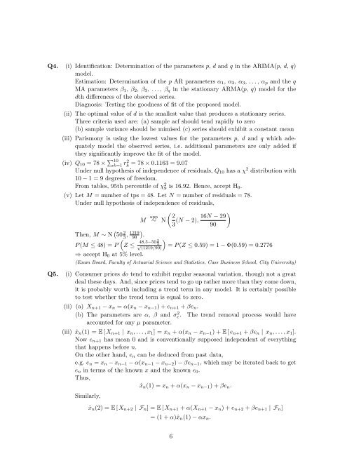
Q4. (i) Identification: Determination of the parameters p, d and q in the ARIMA(p, d, q)
model.
Estimation: Determination of the p AR parameters α 1 , α 2 , α 3 , . . . , α p and the q
MA parameters β 1 , β 2 , β 3 , . . . , β q in the stationary ARMA(p, q) model for the
dth differences of the observed series.
Diagnosis: Testing the goodness of fit of the proposed model.
(ii) The optimal value of d is the smallest value that produces a stationary series.
Three criteria used are: (a) sample acf should tend rapidly <strong>to</strong> zero
(b) sample variance should be mimised (c) series should exhibit a constant mean
(iii) Parismony is using the lowest values for the parameters p, d and q which adequately
model the observed series, i.e. additional parameters are only added if
they significantly improve the fit of the model.
(iv) Q 10 = 78 × ∑ 10
k=1 r2 k
= 78 × 0.1163 = 9.07
Under null hypothesis of independence of residuals, Q 10 has a χ 2 distribution with
10 − 1 = 9 degrees of freedom.
From tables, 95th percentile of χ 2 9 is 16.92. Hence, accept H 0.
(v) Let M = number of tps = 48. Let N = number of residuals = 78.
Under null hypothesis of independence of residuals,
( )
M app 2 16N − 29
∼ N (N − 2),
3 90
Then, M ∼ N ( 50 2 3 , 1219 )
90 .
(
)
P (M ≤ 48) = P Z ≤ 48.5−50 2 √ 3
(1219/90)
= P (Z ≤ 0.59) = 1 − Φ(0.59) = 0.2776
⇒ accept H 0 at 5% level.
(Exam Board, Faculty of Actuarial Science and Statistics, Cass Business School, City University)
Q5. (i) Consumer prices do tend <strong>to</strong> exhibit regular seasonal variation, though not a great
deal these days. And, since prices tend <strong>to</strong> go up rather more than they come down,
it is probably worth including a trend term in any model. It is certainly possible
<strong>to</strong> test whether the trend term is equal <strong>to</strong> zero.
(ii) (a) X n+1 − x n = α(x n − x n−1 ) + e n+1 + βe n .
(b) The parameters are α, β and σe.
2 The trend removal process would have
accounted for any µ parameter.
(iii) ˆx n (1) = E [X n+1 | x n , . . . , x 1 ] = x n + α(x n − x n−1 ) + E [e n+1 + βe n | x n , . . . , x 1 ].
Now e n+1 has mean 0 and is conventionally supposed independent of everything
that happens before n.
On the other hand, e n can be deduced from past data,
e.g. e n = x n − x n−1 − α(x n−1 − x n−2 ) − βe n−1 , which may be iterated back <strong>to</strong> get
e n in terms of the known x and the known e 0 .
Thus,
ˆx n (1) = x n + α(x n − x n−1 ) + βe n .
Similarly,
ˆx n (2) = E [X n+2 | F n ] = E [X n+1 + α(X n+1 − x n ) + e n+2 + βe n+1 | F n ]
= (1 + α)ˆx n (1) − αx n .
6