Bias and Efficiency in fMRI Time-Series Analysis - Purdue University

More documents

Recommendations

Info

fMRI TIME-SERIES ANALYSIS 201 because a large number of scans enter into the estimation in fixed-effect analyses, and random-effects analyses (with fewer degrees of freedom) do not have to contend with serial correlations. FIG. 4. Efficiencies and biases computed according to Eq. (3) and Eq. (4) in the main text for the regressors in Fig. 2 and contrasts of [1 0] and [0 1] for three models of intrinsic correlations [AR(16), AR(1), and the modified 1/f models] and assuming they do not exist (“none”). The results are for the Gauss–Markov estimators (i.e., using a whitening strategy based on the appropriate model in each case) using the first model [AR(16)] as an approximation to the true correlations. The contrast variances have been normalized to the minimum attainable. The bias and increased contrast variance induced result from adopting a whitening strategy when there is a discrepancy between the actual and the assumed intrinsic correlations. and Friston, 1995). Generally if the regressors conform to these eigenvectors then there is no loss of efficiency. The bias incurred by mis-specification can be substantial, resulting in an over- [AR(1)] or under- (1/f and “none”) estimation of the contrast variance leading, in turn, to inexact tests using the associated T statistic that are unduly insensitive [AR(1)] or invalid (1/f and “none”). The effect is not trivial. For example the bias engendered by assuming an AR(1) form in Fig. 4 is about 24%. This would result in about a 10% reduction of T values and could have profound effects on inference. In summary the use of minimum variance, or maximum efficiency, filters can lead to invalid tests. This suggests that the use of whitening is inappropriate and the more important objective is to adopt filtering strategies that minimize bias to ensure that the tests are robust in the face of misspecified autocorrelation structures (i.e., their validity is retained). The minimum bias approach is even more tenable given that sensitivity in fMRI is not generally a great concern. This is Minimum Bias Filters There are two fundamental problems when trying to model intrinsic correlations: (i) one generally does not know the true intrinsic correlations and (ii) even if they were known for any given voxel time series, adopting the same assumptions for all voxels will lead to bias and loss of efficiency because each voxel has a different correlation structure (e.g., brain-stem voxels will be subject to pulsatile effects, ventricular voxels will be subject to CSF flow artifacts, white matter voxels will not be subject to neurogenic noise). It should be noted that very reasonable methods have been proposed for local estimates of spatially varying noise (e.g., Lange and Zeger, 1997). However, in this paper we assume that computational, and other, constraints require us to use the same statistical model for all voxels. One solution to the “bias problem” is described in Worsley and Friston (1995) and involves conditioning the serial correlations by smoothing. This effectively imposes a structure on the intrinsic correlations that renders the difference between the assumed and the actual correlations less severe. Although generally less efficient, the ensuing inferences are less biased and therefore more robust. The loss of efficiency can be minimized by appropriate experimental design and choosing a suitable filter S. In other words there are certain forms of temporal filtering for which SV i S T SV a S T even when V i is not known [see Eq. (4)]. These filters will minimize bias. The problem is to find a suitable form for S. One approach to designing a minimum bias filter is to treat the intrinsic correlation V i , not as an unknown deterministic variable, but as a random variable, whose distributional properties are known or can be estimated. We can then choose a filter that minimizes the expected square bias over all V i , S MB min arg S S S biasS, V i 2 pV i dV i . (5) Equation (5) says that the ideal filter would minimize the expected or mean square bias over all intrinsic correlation structures encountered. An expression for mean square bias and the equivalent mean contrast variance (i.e., 1/efficiency) is provided in Appendix C. This expression uses the first and second order moments of the intrinsic autocorrelation function, parameterized in terms of the underlying autoregression co-
202 FRISTON ET AL. might posit band-pass filtering as a minimum bias filter. In the limit of very narrow band-pass filtering the spectral densities of the assumed and actual correlations, after filtering, would be identical and bias would be negligible. Clearly this would be inefficient but suggests that some band-pass filter might be an appropriate choice. Although there is no single universal minimum bias filter, in the sense it will depend on the design matrix and contrasts employed and other data acquisition parameters; one indication of which frequencies can be usefully attenuated derives from examining how bias depends on the upper and lower cutoff frequencies of a band-pass filter. 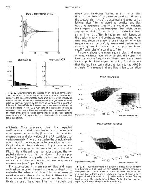Figure 6 shows the mean square bias and mean contrast variance incurred by varying the upper and lower band-pass frequencies. These results are based on the epoch-related regressors in Fig. 2 and assume that the intrinsic correlations conform to the AR(16) estimate. This means that any bias is due to variation FIG. 5. Characterizing the variability in intrinsic correlations. Top: The 16 partial derivatives of the autocorrelation function with respect to the eigenvectors of the covariance matrix of the underlying autoregression coefficients. These represent changes to the autocorrelation function induced by the principal components of variation inherent in the coefficients. The covariances were evaluated over the voxels described in Fig. 2. Lower left: The associated eigenvalue spectrum. Lower right: The autocorrelation function associated with the mean of the autoregression coefficients. These characterizations enter into Eq. (C.3) in Appendix C, to estimate the mean square bias for a given filter. efficients. More precisely, given the expected coefficients and their covariances, a simple secondorder approximation to Eq. (5) obtains in terms of the eigenvectors and eigenvalues of the AR coefficient covariance matrix. These characterize the principal variations about the expected autocorrelation function. Empirical examples are shown in Fig. 5, based on the variation over gray matter voxels in the data used in Fig. 2. Here the principal variations, about the expected autocorrelation function (lower right), are presented (top) in terms of partial derivatives of the autocorrelation function with respect to the autoregressive eigenvectors (see Appendix C). The expressions for mean square bias and mean contrast variance will be used in the next subsection to evaluate the behavior of three filtering schemes in relation to each other and a number of different correlation models. First however, we will use them to motivate the use of band-pass filtering: Intuitively one FIG. 6. Top: Mean square bias (shown in image format in inset) as a function of high- and low-pass cutoff frequencies defining a band-pass filter. Darker areas correspond to lower bias. Note that minimum bias attains when a substantial degree of smoothing or low-pass filtering is used in conjunction with high-pass filtering (dark area on the middle left). Bottom: As for the top but now depicting efficiency. The gray scale is arbitrary.
Page 1 and 2: NeuroImage 12, 196-208 (2000) doi:1
Page 3 and 4: 198 FRISTON ET AL. event-related de
Page 5: 200 FRISTON ET AL. FIG. 3. Spectral
Page 9 and 10: 204 FRISTON ET AL. where S s F (
Page 11 and 12: 206 FRISTON ET AL. DISCUSSION This
Page 13: 208 FRISTON ET AL. BiasS, V i Var

Bias and Efficiency in fMRI Time-Series Analysis - Purdue University

You also want an ePaper? Increase the reach of your titles

Delete template?

Save as template?