Bias and Efficiency in fMRI Time-Series Analysis - Purdue University
Bias and Efficiency in fMRI Time-Series Analysis - Purdue University
Bias and Efficiency in fMRI Time-Series Analysis - Purdue University

You also want an ePaper? Increase the reach of your titles
YUMPU automatically turns print PDFs into web optimized ePapers that Google loves.
204 FRISTON ET AL.<br />
where S s F (1 s)1; 1 is the identity matrix <strong>and</strong><br />
s is varied between 0 (no filter<strong>in</strong>g) <strong>and</strong> 1 (filter<strong>in</strong>g with<br />
F). The models <strong>and</strong> filters considered correspond to<br />
V a V AR(1)<br />
V 1/f <strong>and</strong> F<br />
V AR(16)<br />
V a 1/2 “whiten<strong>in</strong>g”<br />
S H “high-pass”<br />
S L S H “b<strong>and</strong>-pass” .<br />
Mean square bias <strong>and</strong> mean contrast variance are<br />
shown as functions of the filter<strong>in</strong>g parameter s <strong>in</strong> Fig.<br />
9 for the various schema above. The effect on efficiency<br />
is remarkably consistent over the models assumed for<br />
the <strong>in</strong>tr<strong>in</strong>sic correlations. The most efficient filter is a<br />
whiten<strong>in</strong>g filter that progressively decreases the expected<br />
contrast variance. High-pass filter<strong>in</strong>g does not<br />
FIG. 8. The spectral density <strong>and</strong> autocorrelation functions predicted<br />
on the basis of the three models shown <strong>in</strong> Fig. 3, after filter<strong>in</strong>g<br />
with the b<strong>and</strong>-pass filter <strong>in</strong> Fig. 7. Compare these functions with<br />
those <strong>in</strong> Fig. 3. The differences are now ameliorated.<br />
correlations: (i) AR(1), (ii) 1/f, <strong>and</strong> (iii) AR(16). Aga<strong>in</strong><br />
we will assume that the AR(16) estimates are a good<br />
approximation to the true <strong>in</strong>tr<strong>in</strong>sic correlations. For<br />
each model we compared the effect of filter<strong>in</strong>g the data<br />
with whiten<strong>in</strong>g. In order to demonstrate the <strong>in</strong>teraction<br />
between high- <strong>and</strong> low-pass filter<strong>in</strong>g we used a<br />
high-pass filter <strong>and</strong> a b<strong>and</strong>-pass filter. The latter corresponds<br />
to high-pass filter<strong>in</strong>g with smooth<strong>in</strong>g. The<br />
addition of smooth<strong>in</strong>g is the critical issue here: The<br />
high-pass component is motivated by considerations of<br />
both bias <strong>and</strong> efficiency. One might expect that highpass<br />
filter<strong>in</strong>g would decrease bias by remov<strong>in</strong>g low<br />
frequencies that are poorly modeled by simple models.<br />
Furthermore the effect on efficiency will be small because<br />
the m<strong>in</strong>imum variance filter is itself a high-pass<br />
filter. On the other h<strong>and</strong> smooth<strong>in</strong>g is likely to reduce<br />
efficiency markedly <strong>and</strong> its application has to be justified<br />
much more carefully.<br />
The impact of filter<strong>in</strong>g can be illustrated by parametrically<br />
vary<strong>in</strong>g the amount of filter<strong>in</strong>g with a filter F,<br />
FIG. 9. The effect of filter<strong>in</strong>g on mean square bias <strong>and</strong> mean<br />
contrast variance when apply<strong>in</strong>g three filters: the b<strong>and</strong>-pass filter <strong>in</strong><br />
Fig. 8 (solid l<strong>in</strong>es), the high-pass filter <strong>in</strong> Fig. 8 (dashed l<strong>in</strong>es), <strong>and</strong> a<br />
whiten<strong>in</strong>g filter appropriate to the model assumed for the <strong>in</strong>tr<strong>in</strong>sic<br />
correlations (dot–dash l<strong>in</strong>es). Each of these filters was applied under<br />
three models: an AR(1) model (top), a modified 1/f model (middle),<br />
<strong>and</strong> an AR(16) model (bottom). The expected square biases (left) <strong>and</strong><br />
contrast variances (right) were computed as described <strong>in</strong> Appendix C<br />
<strong>and</strong> plotted aga<strong>in</strong>st a parameter s that determ<strong>in</strong>es the degree of<br />
filter<strong>in</strong>g applied (see ma<strong>in</strong> text).