STA 36-786: Bayesian Theoretical Statistics I
STA 36-786: Bayesian Theoretical Statistics I
STA 36-786: Bayesian Theoretical Statistics I

Create successful ePaper yourself
Turn your PDF publications into a flip-book with our unique Google optimized e-Paper software.
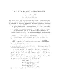
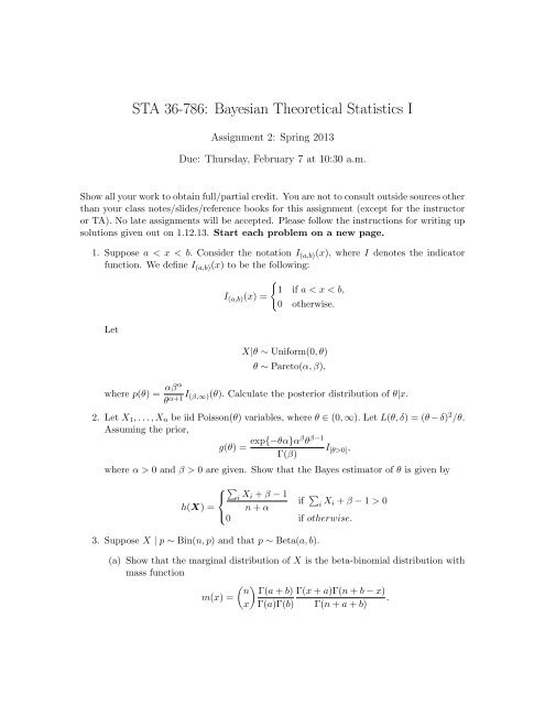
<strong>STA</strong> <strong>36</strong>-<strong>786</strong>: <strong>Bayesian</strong> <strong>Theoretical</strong> <strong>Statistics</strong> I<br />
Assignment 2: Spring 2013<br />
Due: Thursday, February 7 at 10:30 a.m.<br />
Show all your work to obtain full/partial credit. You are not to consult outside sources other<br />
than your class notes/slides/reference books for this assignment (except for the instructor<br />
or TA). No late assignments will be accepted. Please follow the instructions for writing up<br />
solutions given out on 1.12.13. Start each problem on a new page.<br />
1. Suppose a < x < b. Consider the notation I (a,b) (x), where I denotes the indicator<br />
function. We define I (a,b) (x) to be the following:<br />
Let<br />
I (a,b) (x) =<br />
{<br />
1 if a < x < b,<br />
0 otherwise.<br />
X|θ ∼ Uniform(0, θ)<br />
θ ∼ Pareto(α, β),<br />
where p(θ) = αβα<br />
θ α+1 I (β,∞)(θ). Calculate the posterior distribution of θ|x.<br />
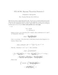
2. Let X 1 , . . . , X n be iid Poisson(θ) variables, where θ ∈ (0, ∞). Let L(θ, δ) = (θ − δ) 2 /θ.<br />
Assuming the prior,<br />
g(θ) = exp{−θα}αβ θ β−1<br />
I<br />
Γ(β) [θ>0] ,<br />
where α > 0 and β > 0 are given. Show that the Bayes estimator of θ is given by<br />
⎧∑<br />
⎨ i X i + β − 1<br />
if ∑ i<br />
h(X) = n + α<br />
X i + β − 1 > 0<br />
⎩<br />
0 if otherwise.<br />
3. Suppose X | p ∼ Bin(n, p) and that p ∼ Beta(a, b).<br />
(a) Show that the marginal distribution of X is the beta-binomial distribution with<br />
mass function<br />
( ) n Γ(a + b) Γ(x + a)Γ(n + b − x)<br />
m(x) =<br />
.<br />
x Γ(a)Γ(b) Γ(n + a + b)
(b) Show that the mean and variance of the beta-binomial is given by EX =<br />
na<br />
( ) ( ) ( )<br />
a + b<br />
a b a + b + n<br />
and VX = n<br />
.<br />
a + b a + b a + b + 1<br />
Hint: For part(b): Use the formulas for iterated expectation and iterated variance.<br />
4. DasGupta (1994) presents an identity relating the Bayes risk to bias, which illustrates<br />
that a small bias can help achieve a small Bayes risk. Let X ∼ f(x|θ) and θ ∼ π(θ).<br />
The Bayes estimator under squared error loss is ˆδ = E(θ|X). Show that the Bayes<br />
risk of ˆδ can be written<br />
∫ ∫<br />
∫<br />
r(π, ˆδ) = [θ − ˆδ(X)] 2 f(x|θ)π(θ)dx dθ = − θ b(θ)π(θ) dθ<br />
Θ X<br />
Θ<br />
where b(θ) = E[ˆδ|θ] − θ is the bias of ˆδ.<br />
5. Suppose that<br />
Using the HB model above,<br />
X|θ ∼ f(x|θ)<br />
θ|λ ∼ π(θ|λ)<br />
λ ∼ π(λ).<br />
(a) prove that E[θ|x] = E[ E[θ|x, λ] ].<br />
(b) prove that V [θ|x] = E[ V [θ|x, λ] ] + V [ E[θ|x, λ] ].<br />
Remark: when proving (a) and (b) above, you may show this two ways, either<br />
by integrals in which say what you are integrating over or you may simply just<br />
use expectations (and in this case specifying what you are taking an expectation<br />
over).<br />
6. Albert and Gupta (1985) investigate theory and application of the hierarchical model<br />
X i |θ i<br />
ind<br />
∼ Bin(n, θ i ), i = 1, . . . , p<br />
θ i |η ∼ Beta(kη, k(1 − η)), k known<br />
η ∼ Uniform(0, 1).<br />
(a) Show that<br />
and<br />
E(θ i |x) =<br />
V (θ i |x) = E[θ i|x](1 − E[θ i |x])<br />
n + k + 1<br />
Hint: You should show along the way that<br />
n x i<br />
n + k n + k<br />
n + k E(η|x)<br />
+<br />
k 2 V (η|x)<br />
(n + k)(n + k + 1) .<br />
V (θ i |x) = x i(n + k − x i ) + E(η|x)k(n + k − 2x i ) − k 2 E(η 2 |x)<br />
(n + k) 2 (n + k + 1)<br />
+ k2 V (η|x)<br />
(n + k) 2 .<br />
General Remark: Note that E(η|x) and V (η|x) are not expressible in a simple<br />
form and hence you can leave them as such.<br />
2
(b) Unconditionally on η, the θ i ’s have conditional covariance<br />
Show this.<br />
Cov(θ i , θ j |x) =<br />
( ) k 2<br />
V (η|x) for i ≠ j.<br />
n + k<br />
(c) Ignoring the prior on η, show how to construct an EB estimator of θ i . Again,<br />
this is not expressible in a simple form. That is, simply derive the marginal<br />
distribution and then explain using software how you would find an estimator<br />
for η. Then give a simple construction for the EB estimator.<br />
3