Chapter 2 Introduction to Bayesian Methods

Chapter 2
Introduction to Bayesian
Methods
Every time I think I know what’s going on, suddenly there’s another layer of
complicitions. I just want this damned thing solved.
—John Scalzi, The Lost Colony
We introduce Bayesian methods first by motivations in decision theory and
introducing the ideas of loss functions, as well as many others. Advanced
topics in decision theory will be covered much later in the course. We will
cover the following topics as well in this chapter:
• hierarchical and empirical Bayesian methods
• the difference between subjective and objective priors
• posterior predictive distributions.
2.1 Decision Theory
Another motivation for the Bayesian approach is decision theory. Its origins
go back to Von Neumann and Morgenstern’s game theory, but the main
character was Wald. In statistical decision theory, we formalize good and
1

2.2 Frequentist Risk 2
bad results with a loss function.
A loss function L(θ, δ(x)) is a function of θ ∈ Θ a parameter or index, and
δ(x) is a decision based on the data x ∈ X. For example, δ(x) = n −1 ∑ n i=1 x i
might be the sample mean, and θ might be the true mean. The loss function
determines the penalty for deciding δ(x) if θ is the true parameter. To give
some intuition, in the discrete case, we might use a 0–1 loss, which assigns
⎧⎪ 0 if δ(x) = θ,
L(θ, δ(x)) = ⎨
⎪⎩
1 if δ(x) ≠ θ,
or in the continuous case, we might use the squared error loss L(θ, δ(x)) =
(θ − δ(x)) 2 . Notice that in general, δ(x) does not necessarily have to be an
estimate of θ. Loss functions provide a very good foundation for statistical
decision theory. They are simply a function of the state of nature (θ) and a
decision function (δ(⋅)). In order to compare procedures we need to calculate
which procedure is best even though we cannot observe the true nature of
the parameter space Θ and data X. This is the main challenge of decision
theory and the break between frequentists and Bayesians.
2.2 Frequentist Risk
Definition 2.1: The frequentist risk is
R(θ, δ(x)) = E θ [L(θ, δ(x))] = ∫ X
L(θ, δ)f(x∣θ) dx.
where θ is held fixed and the expectation is taken over X.
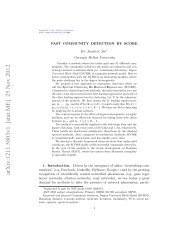
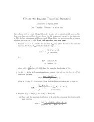
Thus, the risk measures the long-term average loss resulting from using δ.
Figure 1 shows the risk of three different decisions as a function of θ ∈ Θ.
Often one decision does not dominate the other everywhere as is the case
with decisions δ 1 , δ 2 . The challenge is in saying whether, for example, δ 1 or
δ 3 is better. In other words, how should we aggregate over Θ?
Frequentists have a few answers for deciding which is better:

2.2 Frequentist Risk 3
Frequentist Risk
R(θ, δ 1 )
R(θ, δ 2 )
R(θ, δ 3 )
Risk
Figure 2.1: frequentist Risk
Θ
1. Admissibility. A decision which is inadmissible is one that is dominated
everywhere. For example, in Figure 1, δ 2 dominates δ 1 for all
values of θ. It would be easy to compare decisions if all but one were
inadmissible. But usually the risk functions overlap, so this criterion
fails.
2. Restricted classes of procedure. We say that an estimator ˆθ is an
unbiased estimator of θ if E θ [ˆθ] = θ for all θ. If we restrict our attention
to only unbiased estimators then we can often reduce the situation to
only risk curves like δ 1 and δ 2 in Figure 2.2, eliminating overlapping
curves like δ 3 . The existence of an optimal unbiased procedure is a nice
frequentist theory, but many good procedures are biased—for example
Bayesian procedures are typically biased. More surprisingly, some unbiased
procedures are actually inadmissible. For example, James and
Stein showed that the sample mean is an inadmissible estimate of the
mean of a multivariate Gaussian in three or more dimensions. There
are also some problems were no unbiased estimator exists—for example,
when p is a binomial proportion and we wish to estimate 1/p (see
Example 2.1.2 on page 83 of Lehmann and Casella). If we restrict our

2.2 Frequentist Risk 4
class of procedures to those which are equivariant, we also get nice
properties. We do not go into detail here, but these are procedures
with the same group theoretic properties as the data.
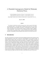
3. Minimax. In this approach we get around the problem by just looking
at sup Θ R(θ, δ(x)), where R(θ, δ(x)) = E θ [L(θ, δ(x))]. For example in
Figure 2, δ 1 would be chosen over δ 2 because its maximum worst-case
risk (the grey dotted line) is lower.
Minimax Frequentist Risk
Risk
R(θ, δ 1 )
R(θ, δ 2 )
Figure 2.2: Minimax frequentist Risk
Θ
A Bayesian answer is to introduce a weighting function p(θ) to tell which
part of Θ is important and integrate with respect to p(θ). In some sense
the frequentist approach is the opposite of the Bayesian approach. However,
sometimes an equivalent Bayesian procedure can be derived using a certain
prior. Before moving on, again note that R(θ, δ(x)) = E θ [L(θ, δ(x))] is
an expectation on X, assuming fixed θ. A Bayesian would only look at x,
the data you observed, not all possible X. An alternative definition of a

2.3 Motivation for Bayes 5
frequentist is, “Someone who is happy to look at other data they could have
gotten but didn’t.”
2.3 Motivation for Bayes
The Bayesian approach can also be motivated by a set of principles. Some
books and classes start with a long list of axioms and principles conceived in
the 1950s and 1960s. However, we will focus on three main principles.
The Bayesian approach can also be motivated by a set of principles. Some
books and classes start with a long list of axioms and principles conceived in
the 1950s and 1960s. However, we will focus on three main principles.
1. Conditionality Principle: The idea here for a Bayesian is that we
condition on the data x.
• Suppose we have an experiment concerning inference about θ that
is chosen from a collection of possible experiments independently.
• Then any experiment not chosen is irrelevant to the inference (this
is the opposite of what we do in frequentist inference).
Example 2.1: For example, two different labs estimate the potency
of drugs. Both have some error or noise in their measurements which
can accurately estimated from past tests. Now we introduce a new
drug. Then we test its potency at a randomly chosen lab. Suppose the
sample sizes matter dramatically.
• Suppose the sample size of the first experiment (lab 1) is 1 and
the sample size of the second experiment (lab 2) is 100.
• What happens if we’re doing a frequentist experiment in terms of
the variance? Since this is a randomized experiment, we need to
take into account all of the data. In essence, the variance will do
some sort of averaging to take into account the sample sizes of
each.
• However, taking a Bayesian approach, we just care about the data
that we see. Thus, the variance calculation will only come from
the actual data at the randomly chosen lab.

2.3 Motivation for Bayes 6
Thus, the question that we ask is should we use the noise level from
the lab where it is tested or average over both? Intuitively, we use the
noise level from the lab where it was tested, but in some frequentist
approaches, it is not always so straightforward.
2. Likelihood Principle: The relevant information in any inference
about θ after observing x is contained entirely in the likelihood function.
Remember the likelihood function p(x∣θ) for fixed x is viewed as
a function of θ, not x. For example in Bayesian approaches, p(θ∣x) ∝
p(x∣θ)p(θ), so clearly inference about θ is based on the likelihood. Another
approach based on the likelihood principle is Fisher’s maximum
likelihood estimation. This approach can also be justified by asymptotics.
In case this principle seems too indisputable, here is an example
using hypothesis testing in coin tossing that shows how some reasonable
procedures may not follow it.
Example 2.2: Let θ be the probability of a particular coin landing on
heads and let
H o ∶ θ = 1/2, H 1 ∶ θ > 1/2.
Now suppose we observe the following sequence of flips:
H,H,T,H,T,H,H,H,H,H,H,T
(9 heads, 3 tails)
Then the likelihood is simply
p(x∣θ) ∝ θ 9 (1 − θ) 3 .
Many non-Bayesian analyses would pick an experimental design that
is reflected in p(x∣θ), for example binomial (toss a coin 12 times) or
negative binomial (toss a coin until you get 3 tails). However the two
lead to different probabilities over the sample space X. This results in
different assumed tail probabilities and p-values.
We repeat a few definitions from mathematical statistics that will be
used in the course at one point or another. For example of sufficient
statistics or distributions that fall in exponential families, we refer the
reader to Theory of Point Estimation (TPE), Chapter 1.

2.3 Motivation for Bayes 7
Definition 2.2: Sufficiency
Recall that for a data set x = (x 1 , . . . , x n ), a sufficient statistic T (x)
is a function such that the likelihood p(x∣θ) = p(x 1 , . . . , x n ∣θ) depends
on x 1 , . . . , x n only through T (x). Then the likelihood p(x∣θ) may be
written as p(x∣θ) = g(θ, T (x)) h(x) for some functions g and h.
Definition 2.3: Exponential Families
A family {P θ } of distributions is said to form an s-dimensional exponential
family if the distributions of P θ have densities of the form
s
p θ (x) = exp [ ∑ η i (θ)T i (x) − B(θ)] h(x).
i=1
3. Sufficiency Principle: The sufficiency principle states that if two different
observations x and y have the same sufficient statistic T (x) =
T (y), then inference based on x and y should be the same. The sufficiency
principle is the least controversial principle.
Theorem 2.1: The posterior distribution, p(θ∣y) only depends on the
data through the sufficient statistic, T(y).
Proof. By the factorization theorem, if T (y) is sufficient,
f(y∣θ) = g(θ, T (y)) h(y).
Then we know the posterior can be written
f(y∣θ)π(θ)
p(θ∣y) =
∫ f(y∣θ)π(θ) dθ
g(θ, T (y)) h(y)π(θ)
=
∫ g(θ, T (y)) h(y)π(θ) dθ
g(θ, T (y))π(θ)
=
∫ g(θ, T (y))π(θ) dθ
∝ g(θ, T (y)) p(θ),
which only depends on y through T (y).
Example 2.3: Sufficiency
Let y ∶= ∑ i y i . Consider
y 1 , . . . , y n ∣θ iid
∼ Bin(1, θ).

2.4 Bayesian Decision Theory 8
Then p(y) = ( n y )θy (1 − θ) n−y . Let p(θ) represent a general prior. Then
p(θ∣y) ∝ θ y (1 − θ) n−y p(θ),
which only depends on the data through the sufficient statistic y.
Theorem 2.2: (Birnbaum).
Sufficiency Principle + Conditionality Principle = Likelihood Principle.
So if we assume the sufficiency principle, then the conditionality and
likelihood principles are equivalent. The Bayesian approach satisfies all
of these principles.
2.4 Bayesian Decision Theory
Earlier we discussed the frequentist approach to statistical decision theory.
Now we discuss the Bayesian approach in which we condition on x and integrate
over Θ (remember it was the other way around in the frequentist approach).
The posterior risk is defined as ρ(π, δ(x)) = ∫ Θ
L(θ, δ(x))π(θ∣x) dθ.
The Bayes action δ ∗ (x) for any fixed x is the decision δ(x) that minimizes
the posterior risk. If the problem at hand is to estimate some unknown
parameter θ, then we typically call this the Bayes estimator instead.
Theorem 2.3: Under squared error loss, the decision δ(x) that minimizes
the posterior risk is the posterior mean.
Proof. Suppose that L(θ, δ(x)) = (θ − δ(x)) 2 . Now note that
ρ(π, δ(x)) = ∫ (θ − δ(x)) 2 π(θ∣x) dθ
= ∫ θ 2 π(θ∣x) dθ + δ(x) 2 ∫ π(θ∣x) dθ − 2δ(x) ∫ θπ(θ∣x) dθ.
Then
∂[ρ(π, δ(x))]
∂[δ(x)]
= 2δ(x) − 2 ∫ θπ(θ∣x) dθ = 0 ⇐⇒ δ(x) = E[θ∣x],
and ∂ 2 [ρ(π, δ(x))]/∂[δ(x)] 2 = 2 > 0, so δ(x) = E[θ∣x] is the minimizer.

2.4 Bayesian Decision Theory 9
Recall that decision theory provides a quantification of what it means for
a procedure to be ‘good.’ This quantification comes from the loss function
L(θ, δ(x)). Frequentists and Bayesians use the loss function differently.
◯
Frequentist Interpretation: Risk
In frequentist usage, the parameter θ is fixed, and thus it is the sample space
over which averages are taken. Letting R(θ, δ(x)) denote the frequentist
risk, recall that R(θ, δ(x)) = E θ [L(θ, δ(x))]. This expectation is taken over
the data X, with the parameter θ held fixed. Note that the data, X, is
capitalized, emphasizing that it is a random variable.
Example 2.4: (Squared error loss). Let the loss function be squared error.
In this case, the risk is
R(θ, δ(x)) = E θ [(θ − δ(x)) 2 ]
= E θ [{θ − E θ [δ(x)] + E θ [δ(x)] − δ(x)} 2 ]
= {θ − E θ [δ(x)]} 2 + E θ [{δ(x) − E θ [δ(x)]} 2
= Bias 2 + Variance
This result allows a frequentist to analyze the variance and bias of an estimator
separately, and can be used to motivate frequentist ideas, e.g. minimum
variance unbiased estimators (MVUEs).
◯
Bayesian Interpretation: Posterior Risk
Bayesians do not find the previous idea compelling because it doesn’t adhere
to the conditionality principle since it averages over all possible data sets.
Hence, in a Bayesian framework, we define the posterior risk ρ(x, π) based
on the data x and a prior π, where
ρ(π, δ(x)) = ∫ Θ
L(θ, δ(x))π(θ∣x) dθ.
Note that the prior enters the equation when calculating the posterior density.
Using the Bayes risk, we can define a bit of jargon. Recall that the Bayes
action δ ∗ (x) is the value of δ(x) that minimizes the posterior risk. We already
showed that the Bayes action under squared error loss is the posterior mean.

2.5 Bayesian Parametric Models 10
◯
Hybrid Ideas
Despite the tensions between frequentists and Bayesians, they occasionally
steal ideas from each other.
Definition 2.4: The Bayes risk is denoted by r(π, δ(x)). While the Bayes
risk is a frequentist concept since it averages over X, the expression can also
be interpreted differently. Consider
r(π, δ(x)) = ∫ ∫ L(θ, δ(x)) f(x∣θ) π(θ) dx dθ
r(π, δ(x)) = ∫ ∫ L(θ, δ(x)) π(θ∣x) π(x) dx dθ
r(π, δ(x)) = ∫ ρ(π, δ(x)) π(x) dx.
Note that the last equation is the posterior risk averaged over the marginal
distribution of x. Another connection with frequentist theory includes that
finding a Bayes rule against the “worst possible prior” gives you a minimax
estimator. While a Bayesian might not find this particularly interesting, it
is useful from a frequentist perspective because it provides a way to compute
the minimax estimator.
We will come back to more decision theory in a more later chapter on advanced
decision theory, where we will cover topics such as minimaxity, admissibility,
and James-Stein estimators.
2.5 Bayesian Parametric Models
For now we will consider parametric models, which means that the parameter
θ is a fixed-dimensional vector of numbers. Let x ∈ X be the observed
data and θ ∈ Θ be the parameter. Note that X may be called the sample
space, while Θ may be called the parameter space. Now we define some

2.5 Bayesian Parametric Models 11
notation that we will reuse throughout the course:
p(x∣θ)
π(θ)
p(x) = ∫ p(x∣θ)π(θ) dθ
p(θ∣x) = p(x∣θ)π(θ)
p(x)
p(x new ∣x) = ∫ p(x new ∣θ)π(θ∣x) dθ
likelihood
prior
marginal likelihood
posterior probability
predictive probability
Most of Bayesian analysis is calculating these quantities in some way or
another. Note that the definition of the predictive probability assumes exchangeability,
but it can easily be modied if the data are not exchangeable.
As a helpful hint, note that for the posterior distribution,
p(θ∣x) = p(x∣θ)π(θ)
p(x)
∝ p(x∣θ)π(θ),
and oftentimes it’s best to not calculate the normalizing constant p(x) because
you can recognize the form of p(x∣θ)π(θ) as a probability distribution
you know. So don’t normalize until the end!
Remark: Note that the prior distribution that we take on θ doesn’t have
to be a proper distribution, however, the posterior is always required to be
proper for valid inference. By proper, I mean that the distribution must
integrate to 1.
Two questions we still need to address are
• How do we choose priors?
• How do we compute the aforementioned quantities, such as posterior
distributions?
We’ll focus on choosing priors for now.

2.6 How to Choose Priors 12
2.6 How to Choose Priors
We will discuss objective and subjective priors. Objective priors may be
obtained from the likelihood or through some type of invariance argument.
Subjective priors are typically arrived at by a process involving interviews
with domain experts and thinking really hard; in fact, there is arguably more
philosophy and psychology in the study of subjective priors than mathematics.
We start with conjugate priors. The main justification for the use of
conjugate priors is that they are computationally convenient and they have
asymptotically desirably properties.
Choosing prior probabilities: Subjective or Objective.
Subjective
A prior probability could be subjective based on the information a person
might have due to past experience, scientific considerations, or simple common
sense. For example, suppose we wish to estimate the probability that a
randomly selected woman has breast cancer. A simple prior could be formulated
based on the national or worldwide incidence of breast cancer. A more
sophisticated approach might take into account the woman’s age, ethnicity,
and family history. Neither approach could necessarily be classified as right
or wrong—again, it’s subjective.
As another example, say a doctor administers a treatment to patients and
finds 48 out of 50 are cured. If the same doctor later wishes to investigate
the cure probability of a similar but slightly different treatment, he might
expect that its cure probability will also be around 48/50 = 0.96. However a
different doctor may have only had 8/10 patients cured by the first treatment
and might therefore specify a prior suggesting a cure rate of around 0.8 for the
for the new treatment. For convenience, subjective priors are often chosen to
take the form of common distributions, such as the normal, gamma, or beta
distribution.
Objective
An objective prior (also called default, vague, noninformative) can also be
used in a given situation even in the absence of enough information. Examples
of objective priors are flat priors such as Laplace’s, Haldane’s, Jeffreys’,
and Bernardo’s references priors. These priors will be discussed later.

2.7 Hierarchical Bayesian Models 13
2.7 Hierarchical Bayesian Models
In a hierarchical Bayesian model, rather than specifying the prior distribution
as a single function, we specify it as a hierarchy. Thus, on the unknown
parameter of interest, say θ, we put a prior. On any other unknown hyperparameters
of the model that are given, we also specify priors for these. We
write
X∣θ ∼ f(x∣θ)
Θ∣γ ∼ π(θ∣γ)
Γ ∼ φ(γ),
where we assume that φ(γ) is known and not dependent on any other unknown
hyperparameters (what the parameters of the prior are often called as
we have already said). Note that we can continue this hierarchical modeling
and add more stages to the model, however note that doing so adds more
complexity to the model (and possibly as we will see may result in a posterior
that we cannot compute without the aid of numerical integration or MCMC,
which we will cover in detail in a later chapter).
Definition 2.5: (Conjugate Distributions). Let F be the class of sampling
distributions p(y∣θ). Then let P denote the class of prior distributions on θ.
Then P is said to be conjugate to F if for every p(θ) ∈ P and p(y∣θ) ∈ F,
p(y∣θ) ∈ P. Simple definition: A family of priors such that, upon being
multiplied by the likelihood, yields a posterior in the same family.
Example 2.5: (Beta-Binomial) If X∣θ is distributed as binomial(n, θ), then
a conjugate prior is the beta family of distributions, where we can show that
the posterior is
π(θ∣x) ∝ p(x∣θ)p(θ)
∝ ( n x )θx n−x
Γ(a + b)
(1 − θ)
Γ(a)Γ(b) θa−1 (1 − θ) b−1
∝ θ x (1 − θ) n−x θ a−1 (1 − θ) b−1
∝ θ x+a−1 (1 − θ) n−x+b−1
⇒
θ∣x ∼ Beta(x + a, n − x + b).

2.7 Hierarchical Bayesian Models 14
Let’s apply this to a real example! We’re interested in the proportion of
people that approve of President Obama in PA.
• We take a random sample of 10 people in PA and find that 6 approve
of President Obama.
• The national approval rating (Zogby poll) of President Obama in mid-
December was 45%. We’ll assume that in MA his approval rating is
approximately 50%.
• Based on this prior information, we’ll use a Beta prior for θ and we’ll
choose a and b. (Won’t get into this here).
• We can plot the prior and likelihood distributions in R and then see
how the two mix to form the posterior distribution.
Density
0.0 0.5 1.0 1.5 2.0 2.5 3.0 3.5
Prior
0.0 0.2 0.4 0.6 0.8 1.0
θ

2.7 Hierarchical Bayesian Models 15
Density
0.0 0.5 1.0 1.5 2.0 2.5 3.0 3.5
Prior
Likelihood
0.0 0.2 0.4 0.6 0.8 1.0
θ
Density
0.0 0.5 1.0 1.5 2.0 2.5 3.0 3.5
Prior
Likelihood
Posterior
0.0 0.2 0.4 0.6 0.8 1.0
θ

2.7 Hierarchical Bayesian Models 16
Example 2.6: (Normal-Uniform Prior)
X 1 , . . . , X n ∣θ iid
∼ Normal(θ, σ 2 ), σ 2 known
θ ∼ Uniform(−∞, ∞),
where θ ∼ Uniform(−∞, ∞) means that p(θ) ∝ 1.
Calculate the posterior distribution of θ given the data.
p(θ∣x) =
=
n
∏
i=1
1 −1
√ exp {
2πσ
2 2σ (x 2 i − θ) 2 }
1 −1
exp {
(2πσ 2 )
n/2
2σ 2
∝ exp { −1
2σ 2 ∑ i
n
∑
i=1
(x i − θ) 2 } .
(x i − θ) 2 }
Note that ∑ i (x i − θ) 2 = ∑ i (x i − ¯x) 2 + n(¯x − θ) 2 . Then
p(θ∣x) ∝ exp { −1
2σ 2 ∑ i
∝ exp { −n
2σ 2 (¯x − θ)2 }
= exp { −n
2σ 2 (θ − ¯x)2 } .
(x i − ¯x) 2 } exp { −n
2σ 2 (¯x − θ)2 }
Thus,
θ∣x 1 , . . . , x n ∼ Normal(¯x, σ 2 /n).
Example 2.7: Normal-Normal
X 1 , . . . , X n ∣θ iid
∼ N(θ, σ 2 )
θ ∼ N(µ, τ 2 ),
where σ 2 is known. Calculate the distribution of θ∣x 1 , . . . , x n .

2.7 Hierarchical Bayesian Models 17
p(θ∣x 1 , . . . , x n ) ∝
n
∏
i=1
1 −1
√ exp {
2πσ
2 2σ (x 2 i − θ) 2 } ×
∝ exp { −1
2σ 2 ∑ i
(x i − θ) 2 } exp { −1
2τ 2 (θ − µ)2 } .
1 −1
√ exp {
2πτ
2 2τ (θ − 2 µ)2 }
Consider
Then
∑
i
(x i − θ) 2 = ∑(x i − ¯x + ¯x − θ) 2 = ∑(x i − ¯x) 2 + n(¯x − θ) 2 .
p(θ∣x 1 , . . . , x n ) = exp { −1
2σ 2 ∑ i
i
i
(x i − ¯x) 2 } × exp { −1
2σ 2 n(¯x − θ)2 } × exp { −1
2τ 2 (θ − µ)2 }
∝ exp { −1
2σ 2 n(¯x − θ)2 } exp { −1
2τ 2 (θ − µ)2 }
= exp { −1
2 [ n σ 2 (¯x2 − 2¯xθ + θ 2 ) + 1
τ 2 (θ2 − 2θµ + µ 2 )]}
= exp { −1
2 [( n σ + 1
2 τ ) 2 θ2 − 2θ ( n¯x
σ + µ 2 τ ) + n¯x2
2 σ + µ2
2 τ ]} 2
⎧⎪
∝ exp ⎨
⎪⎩
⎧⎪
∝ exp ⎨
⎪⎩
−1
2
−1
2
⎡
⎢
( n ⎣
σ + 1
2 τ ) ⎛ n¯x
2 ⎝ θ2 − 2θ
σ 2 + µ ⎤
τ 2 ⎞
⎫⎪
n
σ 2 + 1
τ
⎠
⎬
⎥ 2
⎦
⎪⎭
⎡
⎢
( n ⎣
σ + 1
2 τ ) ⎛ n¯x
2 ⎝ θ − σ 2 + µ 2⎤
τ 2 ⎞ ⎥⎥⎥⎥⎦
⎫ ⎪⎬⎪⎭
n
σ 2 + 1 .
τ
⎠ 2
Recall what it means to complete the square as we did above. 1 Thus,
n¯x
θ∣x 1 , . . . , x n ∼ N ⎛ σ 2 + µ τ 2
n
⎝
σ 2 + 1
τ 2 ,
= N ( n¯xτ 2 + µσ 2
nτ 2 + σ 2 ,
1
n
σ 2 + 1 ⎠
τ 2 ⎞
σ 2 τ 2
nτ 2 + σ 2 ) .
1 Recall from algebra that (x − b) 2 = x 2 − 2bx + b 2 . We want to complete something that
resembles x 2 − 2bx = x 2 + 2bx + (2b/2) 2 − (2b/2) 2 = (x − b) 2 − b 2 .

2.7 Hierarchical Bayesian Models 18
Definition 2.6: The reciprocal of the variance is referred to as the precision.
That is,
1
Precision =
Variance .
Theorem 2.4: Let δ n be a sequence of estimators of g(θ) with mean squared
error E(δ n − g(θ)) 2 .
(i) If E[δ n − g(θ)] 2 → 0 then δ n is consistent for g(θ).
(ii) Equivalent to the above, δ n is consistent if b n (θ) → 0 and V ar(δ n ) → 0
for all θ.
(iii) In particular (and most useful), δ n is consistent if it is unbiased for each
n and if V ar(δ n ) → 0 for all θ.
We omit the proof since it requires Chebychev’s Inequality along with a bit
of probability theory. See Problem 1.8.1 in TPE for the exercise of proving
this.
Example 2.8: (Normal-Normal Revisited) Recall Example 2.7. We write
the posterior mean as E(θ∣x). Let’s write the posterior mean in this example
as
E(θ∣x) =
n¯x
σ 2 + µ τ 2
n
σ 2 + 1
n¯x
σ 2
n
=
σ 2 + 1
We also write the posterior variance as
V (θ∣x) =
τ 2 .
τ 2 +
1
n
σ 2 + 1 .
τ 2
µ
τ 2
n
σ 2 + 1
τ 2 .
We can see that the posterior mean is a weighted average of the sample mean
and the prior mean. The weights are proportional to the reciprocal of the
respective variances (precision). In this case,
1
Posterior Precision =
Posterior Variance
= (n/σ 2 ) + (1/τ 2 )
= Sample Precision + Prior Precision.

2.7 Hierarchical Bayesian Models 19
The posterior precision is larger than either the sample precision or the prior
precision. Equivalently, the posterior variance, denoted by V (θ∣x), is smaller
than either the sample variance or the prior variance.
What happens as n → ∞?
Divide the posterior mean (numerator and denominator) by n. Now take
n → ∞. Then
1 n¯x
E(θ∣x) =
n σ + 1 µ
2 n τ 2
1 n
n σ + 1 →
1
2 n τ 2
¯x
σ 2
1
σ 2 = ¯x as n → ∞.
In the case of the posterior variance, divide the denominator and numerator
by n. Then
V (θ∣x) =
1
n
1 n
n σ + 1 ≈ σ2
1 n 2 n τ 2
→ 0 as n → ∞.
Since the posterior mean is unbiased and the posterior variance goes to 0,
the posterior mean is consistent by Theorem 2.4.

2.7 Hierarchical Bayesian Models 20
Example 2.9:
X∣α, β ∼ Gamma(α, β), α known, β unknown
β ∼ IG(a, b).
Calculate the posterior distribution of β∣x.
p(β∣x) ∝
1
Γ(α)β α xα−1 e −x/β ×
ba
Γ(a) β−a−1 e −b/β
∝ 1
β α e−x/β β −a−1 e −b/β
= β −α−a−1 e −(x+b)/β .
Notice that this looks like an Inverse Gamma distribution with parameters
α + a and x + b. Thus,
β∣x ∼ IG(α + a, x + b).
Example 2.10: (Bayesian versus frequentist)
Suppose a child is given an IQ test and his score is X. We assume that
X∣θ ∼ Normal(θ, 100)
θ ∼ Normal(100, 225)
From previous calculations, we know that the posterior is
θ∣x ∼ Normal (
400 + 9x
, 900
13 13 ) .
Here the posterior mean is (400+9x)/13. Suppose x = 115. Then the posterior
mean becomes 110.4. Contrasting this, we know that the frequentist estimate
is the mle, which is x = 115 in this example.
The posterior variance is 900/13 = 69.23, whereas the variance of the data
is σ 2 = 100.
Now suppose we take the Uniform(−∞, ∞) prior on θ. From an earlier example,
we found that the posterior is
θ∣x ∼ Normal (115, 100) .

2.7 Hierarchical Bayesian Models 21
Notice that the posterior mean and mle are both 115 and the posterior variance
and variance of the data are both 100.
When we put little/no prior information on θ, the data washes away most/all
of the prior information (and the results of frequentist and Bayesian estimation
are similar or equivalent in this case).
Example 2.11: (Normal Example with Unknown Variance)
Consider
X 1 , . . . , X n ∣θ iid
∼ Normal(θ, σ 2 ), θ known, σ 2 unknown
p(σ 2 ) ∝ (σ 2 ) −1 .
Calculate p(σ 2 ∣x 1 , . . . , x n ).
p(σ 2 ∣x 1 , . . . , x n ) ∝ (2πσ 2 ) −n/2 exp { −1
2σ 2 ∑ (x i − θ) 2 } (σ 2 ) −1
i
∝ (σ 2 ) −n/2−1 exp { −1
2σ 2 ∑ (x i − θ) 2 } .
i
Recall, if Y ∼ IG(a, b), then f(y) =
ba
Γ(a) y−a−1 e −b/y . Thus,
σ 2 ∣x 1 , . . . , x n ∼ IG (n/2, ∑n i=1(x i − θ) 2
) .
2
Example 2.12: (Football Data) Gelman et. al (2003) consider the problem
of estimating an unknown variance using American football scores. The focus
is on the difference d between a game outcome (winning score minus losing
score) and a published point spread.
• We observe d 1 , . . . , d n , the observed differences between game outcomes
and point spreads for n = 2240 football games.
• We assume these differences are a random sample from a Normal distribution
with mean 0 and unknown variance σ 2 .
• Our goal is to make inference on the unknown parameter σ 2 , which
represents the variability in the game outcomes and point spreads.

2.7 Hierarchical Bayesian Models 22
We can refer to Example 2.11, since the setup here is the same. Hence the
posterior becomes
σ 2 ∣d 1 , . . . , d n ∼ IG(n/2, ∑ d 2 i /2).
i
The next logical step would be plotting the posterior distribution in R. As far
as I can tell, there is not a built-in function predefined in R for the Inverse
Gamma density. However, someone saw the need for it and built one in using
the pscl package.
Proceeding below, we try and calculate the posterior using the function
densigamma, which corresponds to the Inverse Gamma density. However,
running this line in the code gives the following error:
Warning message:
In densigamma(sigmas, n/2, sum(d^2)/2) : value out of range in ’gammafn’
What’s the problem? Think about the what the posterior looks like. Recall
that
p(σ 2 ∣d) = (∑ i d 2 i /2)n/2
(σ
Γ(n/2)
2 ) −n/2−1 e −(∑ i d 2 i )/2σ2 .
In the calculation R is doing, it’s dividing by Γ(1120), which is a very large
factorial. This is too large for even R to compute, so we’re out of luck here.
So, what can we do to analyze the data?
setwd("~/Desktop/sta4930/football")
data = read.table("football.txt",header=T)
names(data)
attach(data)
score = favorite-underdog
d = score-spread
n = length(d)
hist(d)
install.packages("pscl",repos="http://cran.opensourceresources.org")
library(pscl)
?densigamma
sigmas = seq(10,20,by=0.1)

2.7 Hierarchical Bayesian Models 23
post = densigamma(sigmas,n/2,sum(d^2)/2)
v = sum(d^2)
We know we can’t use the Inverse Gamma density (because of the function in
R), but we do know a relationship regarding the Inverse Gamma and Gamma
distributions. So, let’s apply this fact.
You may be thinking, we’re going to run into the same problem because we’ll
still be dividing by Γ(1120). This is true, except the Gamma density function
dgamma was built into R by the original writers. The dgamma function is able
to do some internal tricks that let it calculate the gamma density even though
the individual piece Γ(n/2) by itself is too large for R to handle. So, moving
forward, we will apply the following fact that we already learned:
If X ∼ IG(a, b), then 1/X ∼ Gamma(a, 1/b).
Since
we know that
σ 2 ∣d 1 , . . . , d n ∼ IG(n/2, ∑ d 2 i /2),
i
1
σ 2 ∣d 1, . . . , d n ∼ Gamma(n/2, 2/v),
where v = ∑ d 2 i .
i
Now we can plot this posterior distribution in R, however in terms of making
inference about σ 2 , this isn’t going to be very useful.
In the code below, we plot the posterior of
1
σ
2 ∣d. In order to do so, we must
create a new sequence of x-values since the mean of our gamma will be at
n/v ≈ 0.0053.
xnew = seq(0.004,0.007,.000001)
pdf("football_sigmainv.pdf", width = 5, height = 4.5)
post.d = dgamma(xnew,n/2,scale = 2/v)
plot(xnew,post.d, type= "l", xlab = expression(1/sigma^2), ylab= "density")
dev.off()
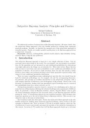
As we can see from the plot below, viewing the posterior of
1
σ
2 ∣d isn’t very
useful. We would like to get the parameter in terms of σ 2 , so that we could

2.7 Hierarchical Bayesian Models 24
density
0 500 1000 2000
0.0040 0.0050 0.0060 0.0070
1 σ 2
Figure 2.3: Posterior Distribution p( 1
σ 2 ∣d 1 , . . . , d n )
plot the posterior distribution of interest as well as calculate the posterior
mean and variance.
To recap, we know
1
σ 2 ∣d 1, . . . , d n ∼ Gamma(n/2, 2/v),
where v = ∑ d 2 i .
i
Let u = 1
σ 2 . We are going to make a transformation of variables now to write
the density in terms of σ 2 .
Since u =
σ 1
2 , this implies σ 2 = 1 ∂u
u
. Then ∣
∂σ ∣ = 1 2 σ . 4
Now applying the transformation of variables we find that
Thus,
f(σ 2 ∣d 1 , . . . , d n ) =
1
Γ(n/2)(2/v) n/2 ( 1 σ 2 ) n/2−1
e − v
2σ 2 ( 1 σ 4 ) .
σ 2 ∣d ∼ Gamma(n/2, 2/v) ( 1 σ 4 ) .

2.7 Hierarchical Bayesian Models 25
Now, we know the density of σ 2 ∣d in a form we can calculate in R.
x.s = seq(150,250,1)
pdf("football_sigma.pdf", height = 5, width = 4.5)
post.s = dgamma(1/x.s,n/2, scale = 2/v)*(1/x.s^2)
plot(x.s,post.s, type="l", xlab = expression(sigma^2), ylab="density")
dev.off()
detach(data)
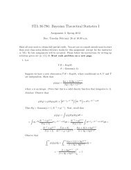
From the posterior plot in Figure 2.4 we can see that the posterior mean is
around 185. This means that the variability of the actual game result around
the point spread has a standard deviation around 14 points. If you wanted to
actually calculate the posterior mean and variance, you could do this using
a numerical method in R.
What’s interesting about this example is that there is a lot more variability
in football games than the average person would most likely think.
• Assume that (1) the standard deviation actually is 14 points, and (2)
game result is normally distributed (which it’s not, exactly, but this is
a reasonable approximation).
• Things with a normal distribution fall two or more standard deviations
from their mean about 5% of the time, so this means that, roughly
speaking, about 5% of football games end up 28 or more points away
from their spread.

2.7 Hierarchical Bayesian Models 26
density
0.00 0.02 0.04 0.06
160 180 200 220 240
Figure 2.4: Posterior Distribution p(σ 2 ∣d 1 , . . . , d n )
σ 2

2.7 Hierarchical Bayesian Models 27
Example 2.13:
Y 1 , . . . , Y n ∣µ, σ 2 iid
∼ Normal(µ, σ 2 ),
µ∣σ 2 ∼ Normal(µ 0 , σ2
κ 0
),
σ 2 ∼ IG( ν 0
2 , σ2 0
2 ),
where µ 0 , κ 0 , ν 0 , σ 2 0
are constant.
Find p(µ, σ 2 ∣y 1 . . . , y n ). Notice that
p(µ, σ 2 ∣y 1 . . . , y n ) = p(µ, σ2 , y 1 . . . , y n )
p(y 1 . . . , y n )
∝ p(y 1 . . . , y n ∣µ, σ 2 )p(µ, σ 2 )
= p(y 1 . . . , y n ∣µ, σ 2 )p(µ∣σ 2 )p(σ 2 ).
Then
p(µ, σ 2 ∣y 1 . . . , y n ) ∝ p(y 1 . . . , y n ∣µ, σ 2 )p(µ∣σ 2 )p(σ 2 )
∝ (σ 2 ) −n/2 exp { −1
2σ 2
n
∑
i=1
× (σ 2 ) −ν 0/2−1 exp { −σ2 0
2σ 2 } .
Consider ∑ i (y i − µ) 2 = ∑ i (y i − ȳ) 2 + n(ȳ − µ) 2 .
Then
(y i − µ) 2 } (σ 2 ) −1/2 exp { −κ 0
2σ (µ − µ 0) 2 }
2
n(ȳ − µ) 2 + κ 0 (µ − µ 0 ) 2 = nȳ 2 − 2nȳµ + nµ 2 + κ 0 µ 2 − 2κ 0 µµ 0 + κ 0 µ 0
2
= (n + κ 0 )µ 2 − 2(nȳ + κ 0 µ 0 )µ + nȳ 2 + κ 0 µ 0
2
= (n + κ 0 ) (µ − nȳ + κ 0µ 0
n + κ 0
)
2
− (nȳ + κ 0µ 0 ) 2
n + κ 0
+ nȳ 2 + κ 0 µ 0 2 .

2.7 Hierarchical Bayesian Models 28
Now consider
nȳ 2 + κ 0 µ 0 2 − (nȳ + κ 0µ 0 ) 2
n + κ 0
= nȳ 2 + κ 0 µ 0 2 + −n2 ȳ 2 − 2nκ 0 µ 0 ȳ − κ 02 µ 0
2
n + κ 0
= n2 ȳ 2 + nκ 0 µ 02 + nκ 0 ȳ 2 + κ 02 µ 02 − n 2 ȳ 2 − 2nκ 0 µ 0 ȳ − κ 02 µ 0
2
n + κ 0
= nκ 0µ 02 + nκ 0 ȳ 2 − 2nκ 0 µ 0 ȳ
n + κ 0
= nκ 0(µ 02 − 2µ 0 ȳ + ȳ 2 )
n + κ 0
= nκ 0(µ 0 − ȳ) 2
n + κ 0
.
Putting this all together, we find
p(µ, σ 2 ∣y 1 . . . , y n ) ∝ exp { −n
2σ 2 (ȳ − µ)2 } exp { −1
2σ 2 ∑ i
× exp { −κ 0
2σ 2 ∑ i
(y i − ȳ) 2 }
(µ − µ 0 ) 2 } (σ 2 ) −n/2−1/2 (σ 2 ) −ν 0/2−1 exp { −σ2 0
2σ 2 }
−nκ 0
= exp {
2σ 2 (n + κ 0 ) (µ 0 − ȳ) 2 } exp { −1
2σ 2 ∑ (y i − ȳ) 2 }
i
× exp {− (n + κ 0)
(µ − nȳ + κ 2
0µ 0
) } (σ
2σ 2 n + κ 2 ) −ν0/2−1 (σ 2 ) −n/2−1 exp { −σ2 0
0 2σ } 2
= exp { −1
2σ 2 ∑ i
(y i − ȳ) 2 −
× exp {− (n + κ 0)
(µ − nȳ + κ 2
0µ 0
) } (σ
2σ 2 n + κ 2 ) −1/2 .
0
Since the posterior above factors, we find
µ∣σ 2 , y ∼ Normal ( nȳ + κ 0µ 0 σ
,
2
) ,
n + κ 0 n + κ 0
nκ 0
2σ 2 (n + κ 0 ) (µ 0 − ȳ) 2 − σ2 0
2σ 2 } (σ2 ) −(n+ν 0)/2−1
σ 2 ∣y ∼ IG ( n + ν 0
, 1 2 2 (∑ i
(y i − ȳ) 2 +
nκ 0
(n + κ 0 ) (µ 0 − ȳ) 2 + σ 2 0 )) .

2.7 Hierarchical Bayesian Models 29
Example 2.14: Suppose we calculate E[θ∣y] where y = x (n) . Let
X i ∣ θ ∼ Uniform(0, θ)
θ ∼ Gamma(a, 1/b).
Show
E[θ∣x] =
1 P (χ 2 < 2/(by))
2(n+a−1)
b(n + a − 1) P (χ 2 < 2/(by)).
2(n+a−1)
Proof. Recall that the posterior depends on the data only through the sufficient
statistic y. Consider that P (Y ≤ y) = P (X 1 ≤ y) n = (y/θ) n ⇒ f y (y) =
n/θ(y/θ) n−1 = n θ n yn−1 .
E[θ∣x] = ∫ θf(y∣θ)π(θ) dθ
∫ f(y∣θ)π(θ) dθ
θ n y n−1 θ −a−1 e −1/(θb)
=
∫ ∞
y
= ∫ ∞
y
∫ ∞
y
θ n Γ(a)b a dθ
nθ a−1 e −1/(θb)
θ n Γ(a)b a dθ
θ −n−a e −1/(θb) dθ
∫ ∞
y
θ −n−a−1 e −1/(θb) dθ
Let θ = 2/(xb) ⇒ dθ = −2/(bx 2 ) dx. Recall that Gamma(v/2, 2) is a χ 2 v.

2.8 Empirical Bayesian Models 30
Then
2
E[θ∣x] = ∫ by
0
( 2 xb )−n−a e −x/2 2
=
2
by
bx 2
∫0 ( 2 xb )−n−a−1 e −x/2 2
2
by
bx 2
dx
dx
∫0 b n+a−1 x n+a−2 e −x/2 dx × Γ(n + a − 1) dx
2 n+a−1 Γ(n + a − 1)
2
by
∫0 b n+a+1−1 x n+a+1−2 e −x/2 dx × Γ(n + a) dx
2 n+a+1−1 Γ(n + a)
= P (χ2 < 2/(by))
2(n+a−1) b n+a−1 Γ(n + a − 1)
P (χ 2 < 2/(by)) b
2(n+a−1) n+a Γ(n + a)
1 P (χ 2
=
< 2/(by))
2(n+a−1)
b(n + a − 1) P (χ 2 < 2/(by)).
2(n+a−1)
2.8 Empirical Bayesian Models
Another generalization of Bayes estimation is called empirical Bayes (EB)
estimation, which most consider to fall outside of the Bayesian paradigm (in
the sense that it’s not fully Bayesian). However, it’s been proved to be a
technique of constructing estimators that perform well under both Bayesian
and frequentist criteria. One reason for this is that EB estimators tend to
be more robust against model misspecification of the prior distribution.
We start again with an HB model, however this time we assume that γ is
unknown and must be estimated. We begin with the Bayes model
X i ∣θ ∼ f(x∣θ), i = 1 . . . , p
Θ∣γ ∼ π(θ∣γ).
We then calculate the marginal distribution of X with density
m(x∣γ) = ∫ ∏ f(x i ∣θ)π(θ∣γ) dθ.

2.8 Empirical Bayesian Models 31
Based on m(x∣γ), we obtain an estimate of ˆγ(x) of γ. It’s most common to
find the estimate using maximum likelihood estimation (MLE), but method
of moments could be used as well (or other methods). We now substitute
ˆγ(x) for γ in π(θ∣γ) and determine the estimator that minimizes the empirical
posterior loss
∫ L(θ, δ)π(θ∣ˆγ(x)) dθ.
Remark: An alternative definition is obtained by substituting ˆγ(x) for γ
in the Bayes estimator. (This proof is left as a homework exercise, 4.6.1 in
TPE).
Example 2.15: Empirical Bayes Binomial
Suppose there are K different groups of patients where each group has n
patients. Each group is given a different treatment for the same illness and
in the kth group, we count X k , k = 1, . . . , K, which is the number of successful
treatments our of n.
Since the groups receive different treatments, we expect different success
rates, however, since we are treating the same illness, these rates should be
related to each other. These considerations suggest the following model:
X k ∼ Bin(n, p k ),
p k ∼ Beta(a, b),
where the K groups are tied together by the common prior distribution.
It is easy to show that the Bayes estimator of p k under squared error loss is
E(p k ∣a k , a, b) =
a + x k
a + b + n .
Suppose now that we are told that a, b are unknown and we wish to estimate

2.9 Posterior Predictive Distributions 32
them using EB. We first calculate
K
m(x∣a, b) = ∫ . . .
0,1
∫ ∏ ( n )p x k
k 0,1 x (1 − p k) n−x k
Γ(a + b)
×
k Γ(a)Γ(b) pa−1 k (1 − p k ) b−1 dp k
k=1
K
= ∫ . . .
0,1
∫ ∏ ( n Γ(a + b)
)
0,1 x k Γ(a)Γ(b) px k+a−1
k
(1 − p k ) n−xk+b−1 dp k
=
K
∏
k=1
k=1
( n x k
) Γ(a + b)Γ(a + x k)Γ(n − x k + b)
Γ(a)Γ(b)Γ(a + b + n)
which is a product of beta-binomials. Although the MLEs of a and b aren’t
expressible in closed form, they can be calculated numerically to construct
the EB estimator
ˆδ EB (x) = â + x k
â + ˆb + n .
2.9 Posterior Predictive Distributions
We have just gone through many examples illustrating how to calculate many
simple posterior distributions. This is the main goal of a Bayesian analysis.
Another goal might be prediction. That is given some data y and a new
observation ỹ, we may wish to find the conditional distribution of ỹ given y.
This distribution is referred to as the posterior predictive distribution. That
is, our goal is to find p(ỹ∣y). This minimizing estimator is called the empirical
Bayes estimator.
We’ll derive the posterior predictive distribution for the discrete case (θ is
discrete). It’s the same for the continuous case, with the sums replaced with
integrals.

2.9 Posterior Predictive Distributions 33
Consider
p(ỹ, y)
p(ỹ∣y) =
p(y)
= ∫ θ p(ỹ, y, θ) dθ
p(y)
= ∫ θ p(ỹ∣y, θ)p(y, θ) dθ
p(y)
= ∫ θ
p(ỹ∣y, θ)p(θ∣y) dθ.
In most contexts, if θ is given, then ỹ∣θ is independent of y, i.e., the value
of θ determines the distribution of ỹ, without needing to also know y. When
this is the case, we say that ỹ and y are conditionally independent given θ.
Then the above becomes
p(ỹ∣y) = ∫ θ
p(ỹ∣θ)p(θ∣y) dθ.
Theorem 2.5: If θ is discrete and ỹ and y are conditionally independent
given θ, then the posterior predictive distribution is
p(ỹ∣y) = ∑ p(ỹ∣θ)p(θ∣y).
θ
If θ is continuous and ỹ and y are conditionally independent given θ, then
the posterior predictive distribution is
p(ỹ∣y) = ∫ θ
p(ỹ∣θ)p(θ∣y) dθ.

2.9 Posterior Predictive Distributions 34
Theorem 2.6: Suppose p(x) is a pdf that looks like p(x) = cf(x), where c
is a constant and f is a continuous function of x. Since
∫ x
p(x) dx = ∫ x
cf(x) dx = 1,
then
∫ x
f(x)dx = 1/c.
Note: No calculus is needed to compute ∫ x
f(x) dx if f(x) looks like a known
pdf.
Example 2.16: Human males have one X-chromosome and one Y-chromosome,
whereas females have two X-chromosomes, each chromosome being inherited
from one parent. Hemophilia is a disease that exhibits X-chromosome-linked
recessive inheritance, meaning that a male who inherits the gene that causes
the disease on the X-chromosome is affected, whereas a female carrying the
gene on only one of her X-chromosomes is not affected. The disease is generally
fatal for women who inherit two such genes, and this is very rare, since
the frequency of occurrence of the gene is very low in human populations.
Consider a woman who has an affected brother (xY), which implies that her
mother must be a carrier of the hemophilia gene (xX). We are also told that
her father is not affected (XY), thus the woman herself has a fifty-fifty chance
of having the gene.
Let θ denote the state of the woman. It can take two values: the woman is
a carrier (θ = 1) or not (θ = 0). Based on this, the prior can be written as
P (θ = 1) = P (θ = 0) = 1/2.
Suppose the woman has a son who does not have hemophilia (S1 = 0). Now
suppose the woman has another son. Calculate the probability that this
second son also will not have hemophilia (S2 = 0), given that the first son
does not have hemophilia. Assume son one and son two are conditionally
independent given θ.
Solution:
p(S2 = 0∣S1 = 0) = ∑ p(S2 = 0∣θ)p(θ∣S1 = 0).
θ

2.9 Posterior Predictive Distributions 35
First compute
Then
p(S1 = 0∣θ)p(θ)
p(θ∣S1 = 0) =
p(S1 = 0∣θ = 0)p(θ = 0) + p(S1 = 0∣θ = 1)p(θ = 1)
(1)(1/2)
⎧⎪ (1)(1/2)+(1/2)(1/2)
= ⎨
= 2 3
if θ = 0
1
⎪⎩ 3
if θ = 1.
p(S2 = 0∣S1 = 0) = p(S2 = 0∣θ = 0)p(θ = 0∣S1 = 0) + p(S2 = 0∣θ = 1)p(θ = 1∣S1 = 0)
= (1)(2/3) + (1/2)(1/3) = 5/6.
Negative Binomial Distribution
Before doing the next example, we will introduce the Negative Binomial
distribution. The binomial distribution counts the numbers of successes in
a fixed number of iid Bernoulli trials. Recall, a Bernoulli trial has a fixed
success probability p.
Suppose instead that we count the number of Bernoulli trials required to get
a fixed number of successes. This formulation leads to the Negative Binomial
distribution.
In a sequence of independent Bernoulli(p) trials, let X denote the trial at
which the rth success occurs, where r is a fixed integer.
Then
f(x) = ( x − 1
r − 1 ) pr (1 − p) x−r , x = r, r + 1, . . .
and we say X ∼ Negative Binom(r, p).
There is another useful formulation of the Negative Binomial distribution.
In many cases, it is defined as Y = number of failures before the rth success.
This formulation is statistically equivalent to the one given above in term of
X = trial at which the rth success occurs, since Y = X − r. Then
f(y) = ( r + y − 1 ) p r (1 − p) y , y = 0, 1, 2, . . .
y
and we say Y ∼ Negative Binom(r, p).
When we refer to the Negative Binomial distribution in this class, we will
refer to the second one defined unless we indicate otherwise.

2.9 Posterior Predictive Distributions 36
Example 2.17: (Poisson-Gamma)
X∣λ ∼ Poisson(λ)
λ ∼ Gamma(a, b)
Assume that ˜X∣λ ∼ Poisson(λ) is independent of X. Assume we have a new
observation ˜x. Find the posterior predictive distribution, p(˜x∣x). Assume
that a is an integer.
Solution:
First, we must find p(λ∣x).
Recall
p(λ∣x) ∝ p(x∣λ)(p(λ)
∝ e −λ λ x λ a−1 e −λ/b
= λ x+a−1 e −λ(1+1/b) .
Thus, λ∣x ∼ Gamma(x + a,
1
1+1/b ), i.e., λ∣x ∼ Gamma(x + a, b
b+1 ).

2.9 Posterior Predictive Distributions 37
It then follows that
p(˜x∣x) = ∫ λ
p(˜x∣λ)p(λ∣x) dλ
e−λλ˜x
1
= ∫ λ ˜x! Γ(x + a)( b λx+a−1 e −λ(b+1)/b dλ
b+1 )x+a
1
=
˜x! Γ(x + a)( b ∫ λ˜x+x+a−1 e −λ(2b+1/b) dλ
b+1 )x+a λ
1
=
Γ(˜x + x + a)(b/(2b + 1)˜x+x+a
˜x! Γ(x + a)( b
b+1
)x+a
Γ(˜x + x + a)(b/(2b + 1)˜x+x+a
=
=
=
˜x! Γ(x + a)( b
b+1 )x+a
Γ(˜x + x + a) b ˜x+x+a (b + 1) x+a
˜x! Γ(x + a) b x+a (2b + 1) ˜x+x+a
( ˜x + x + a − 1)! b˜x (b + 1) x+a
(x + a − 1)! ˜x! (2b + 1)˜x+x+a
= ( ˜x + x + a − 1 ) (
˜x
b
)˜x
2b + 1
( b + 1
2b + 1 ) x+a
.
Let p = b/(2b + 1), which implies 1 − p = (b + 1)/(2b + 1).
Then
Thus,
p(˜x∣x) = ( ˜x + x + a − 1
)p˜x (1 − p) x+a .
˜x
˜x∣x ∼ Negative Binom (x + a,
b
2b + 1 ) .

2.9 Posterior Predictive Distributions 38
Example 2.18: Suppose that X is the number of pregnant women arriving
at a particular hospital to deliver their babies during a given month. The
discrete count nature of the data plus its natural interpretation as an arrival
rate suggest modeling it with a Poisson likelihood.
To use a Bayesian analysis, we require a prior distribution for θ having support
on the positive real line. A convenient choice is given by the Gamma
distribution, since it’s conjugate for the Poisson likelihood.
The model is given by
X∣λ ∼ Poisson(λ)
λ ∼ Gamma(a, b).
We are also told 42 moms are observed arriving at the particular hospital
during December 2007. Using prior study information given, we are told
a = 5 and b = 6. (We found a, b by working backwards from a prior mean
of 30 and prior variance of 180).
We would like to find several things in this example:
1. Plot the likelihood, prior, and posterior distributions as functions of λ
in R.
2. Plot the posterior predictive distribution where the number of pregnant
women arriving falls between [0,100], integer valued.
3. Find the posterior predictive probability that the number of pregnant
women arrive is between 40 and 45 (inclusive).
Solution: The first thing we need to know to do this problem are p(λ∣x) and
p(˜x∣x). We found these in Example 2.17. So,
and
λ∣x ∼ Gamma (x + a,
˜x∣x ∼ Negative Binom (x + a,
b
b + 1 ) ,
b
2b + 1 ) .

2.9 Posterior Predictive Distributions 39
Next, we can move right into R for our analysis.
setwd("~/Desktop/sta4930/ch3")
lam = seq(0,100, length=500)
x = 42
a = 5
b = 6
like = dgamma(lam,x+1,scale=1)
prior = dgamma(lam,5,scale=6)
post = dgamma(lam,x+a,scale=b/(b+1))
pdf("preg.pdf", width = 5, height = 4.5)
plot(lam, post, xlab = expression(lambda), ylab= "Density", lty=2, lwd=3, type="l")
lines(lam,like, lty=1,lwd=3)
lines(lam,prior, lty=3,lwd=3)
legend(70,.06,c("Prior", "Likelihood","Posterior"), lty = c(2,1,3),
lwd=c(3,3,3))
dev.off()
##posterior predictive distribution
xnew = seq(0,100) ## will all be ints
post_pred_values = dnbinom(xnew,x+a,b/(2*b+1))
plot(xnew, post_pred_values, type="h", xlab = "x", ylab="Posterior Predictive Distribution")
## what is posterior predictive prob that number
of pregnant women arrive is between 40 and 45 (inclusive)
(ans = sum(post_pred_values[41:46])) ##recall we included 0
In the first part of the code, we plot the posterior, likelihood, and posterior.
This should be self-explanatory since we have already done an example.
When we find our posterior predictive distribution, we must create a sequence
of integers from 0 to 100 (inclusive) using the seq command. Then we find the
posterior predictive values using the function dnbinom. Then we simply plot
the sequence of x new on the x-axis and the corresponding posterior predictive
values on the y-axis. We set type="h" so that our plot will appear somewhat
like a smooth histogram.
Finally, in order to calculate the posterior predictive probability that the
number of pregnant women who arrive is between 40 and 45, we simply add
up the posterior predictive probabilities that correspond to these values. We
find that the posterior predictive probability of 0.1284 that the number of
pregnant women who arrive is between 40 and 45.