Pricing Asian Options in a Semimartingale Model - Department of ...
Pricing Asian Options in a Semimartingale Model - Department of ...
Pricing Asian Options in a Semimartingale Model - Department of ...

You also want an ePaper? Increase the reach of your titles
YUMPU automatically turns print PDFs into web optimized ePapers that Google loves.
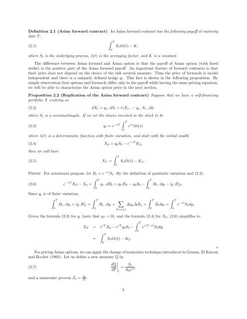
Def<strong>in</strong>ition 2.1 (<strong>Asian</strong> forward contract) An <strong>Asian</strong> forward contract has the follow<strong>in</strong>g pay<strong>of</strong>f at maturity<br />
date T :<br />
(2.1)<br />
∫ T<br />
0<br />
S t dλ(t) − K,<br />
where S t is the underly<strong>in</strong>g process, λ(t) is the averag<strong>in</strong>g factor, and K is a constant.<br />
The difference between <strong>Asian</strong> forward and <strong>Asian</strong> option is that the pay<strong>of</strong>f <strong>of</strong> <strong>Asian</strong> option (with fixed<br />
strike) is the positive part <strong>of</strong> the <strong>Asian</strong> forward pay<strong>of</strong>f. An important feature <strong>of</strong> forward contracts is that<br />
their price does not depend on the choice <strong>of</strong> the risk neutral measure. Thus the price <strong>of</strong> forwards is model<br />
<strong>in</strong>dependent and there is a uniquely def<strong>in</strong>ed hedge q t . This fact is shown <strong>in</strong> the follow<strong>in</strong>g proposition. By<br />
simple observation that options and forwards differ only <strong>in</strong> the pay<strong>of</strong>f while hav<strong>in</strong>g the same pric<strong>in</strong>g equation,<br />
we will be able to characterize the <strong>Asian</strong> option price <strong>in</strong> the next section.<br />
Proposition 2.2 (Replication <strong>of</strong> the <strong>Asian</strong> forward contract) Suppose that we have a self-f<strong>in</strong>anc<strong>in</strong>g<br />
portfolio X evolv<strong>in</strong>g as<br />
(2.2) dX t = q t− dS t + r(X t− − q t− S t− )dt,<br />
where S t is a semimart<strong>in</strong>gale. If we set the shares <strong>in</strong>vested <strong>in</strong> the stock to be<br />
∫ T<br />
(2.3) q t = e −rT e rs dλ(s)<br />
where λ(t) is a determ<strong>in</strong>istic function with f<strong>in</strong>ite variation, and start with the <strong>in</strong>itial wealth<br />
(2.4) X 0 = q 0 S 0 − e −rT K 2 ,<br />
then we will have<br />
(2.5) X T =<br />
∫ T<br />
0<br />
t<br />
S t dλ(t) − K 2 .<br />
Pro<strong>of</strong>. For notational purpose, let B t = e −rt S t . By the def<strong>in</strong>ition <strong>of</strong> quadratic variation and (2.2),<br />
(2.6) e −rT X T − X 0 =<br />
S<strong>in</strong>ce q t is <strong>of</strong> f<strong>in</strong>ite variation,<br />
∫ T<br />
0<br />
B t− dq t + [q, B] t =<br />
∫ T<br />
0<br />
∫ T<br />
0<br />
q t− dB t = q T B T − q 0 S 0 −<br />
B t− dq t + ∑<br />
0