Pricing Asian Options in a Semimartingale Model - Department of ...
Pricing Asian Options in a Semimartingale Model - Department of ...
Pricing Asian Options in a Semimartingale Model - Department of ...

You also want an ePaper? Increase the reach of your titles
YUMPU automatically turns print PDFs into web optimized ePapers that Google loves.
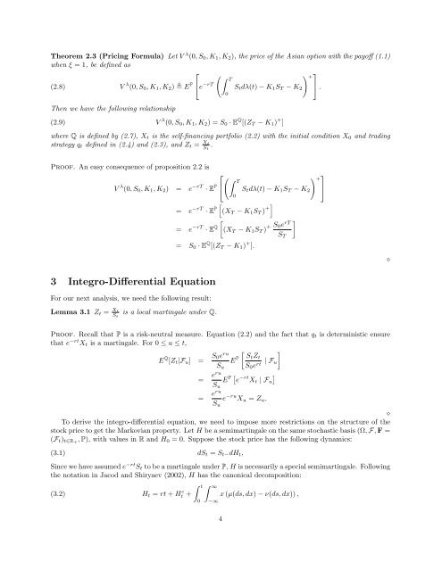
Theorem 2.3 (<strong>Pric<strong>in</strong>g</strong> Formula) Let V λ (0, S 0 , K 1 , K 2 ), the price <strong>of</strong> the <strong>Asian</strong> option with the pay<strong>of</strong>f (1.1)<br />
when ξ = 1, be def<strong>in</strong>ed as<br />
⎡ ( ∫ ) ⎤ + T<br />
(2.8) V λ (0, S 0 , K 1 , K 2 ) E P ⎣e −rT S t dλ(t) − K 1 S T − K 2<br />
⎦ .<br />
Then we have the follow<strong>in</strong>g relationship<br />
(2.9) V λ (0, S 0 , K 1 , K 2 ) = S 0 · E Q [(Z T − K 1 ) + ]<br />
where Q is def<strong>in</strong>ed by (2.7), X t is the self-f<strong>in</strong>anc<strong>in</strong>g portfolio (2.2) with the <strong>in</strong>itial condition X 0 and trad<strong>in</strong>g<br />
strategy q t def<strong>in</strong>ed <strong>in</strong> (2.4) and (2.3), and Z t = Xt<br />
S t<br />
.<br />
0<br />
Pro<strong>of</strong>. An easy consequence <strong>of</strong> proposition 2.2 is<br />
⎡( ∫ T<br />
V λ (0, S 0 , K 1 , K 2 ) = e −rT · E P ⎣<br />
0<br />
) ⎤ +<br />
S t dλ(t) − K 1 S T − K 2<br />
⎦<br />
= e −rT · E P [ (X T − K 1 S T ) +]<br />
= e −rT · E Q [<br />
(X T − K 1 S T ) + S 0 e rT<br />
S T<br />
]<br />
= S 0 · E Q [(Z T − K 1 ) + ].<br />
⋄<br />
3 Integro-Differential Equation<br />
For our next analysis, we need the follow<strong>in</strong>g result:<br />
Lemma 3.1 Z t = Xt<br />
S t<br />
is a local mart<strong>in</strong>gale under Q.<br />
Pro<strong>of</strong>. Recall that P is a risk-neutral measure. Equation (2.2) and the fact that q t is determ<strong>in</strong>istic ensure<br />
that e −rt X t is a mart<strong>in</strong>gale. For 0 ≤ u ≤ t,<br />
E Q [Z t |F u ] = S 0e ru [ ]<br />
E P St Z t<br />
S 0 e rt | F u<br />
S u<br />
= eru<br />
S u<br />
E P [ e −rt X t | F u<br />
]<br />
= eru<br />
e −ru X u = Z u .<br />
S u<br />
⋄<br />
To derive the <strong>in</strong>tegro-differential equation, we need to impose more restrictions on the structure <strong>of</strong> the<br />
stock price to get the Markovian property. Let H be a semimart<strong>in</strong>gale on the same stochastic basis (Ω, F, F =<br />
(F t ) t∈R+ , P), with values <strong>in</strong> R and H 0 = 0. Suppose the stock price has the follow<strong>in</strong>g dynamics:<br />
(3.1) dS t = S t− dH t ,<br />
S<strong>in</strong>ce we have assumed e −rt S t to be a mart<strong>in</strong>gale under P, H is necessarily a special semimart<strong>in</strong>gale. Follow<strong>in</strong>g<br />
the notation <strong>in</strong> Jacod and Shiryaev (2002), H has the canonical decomposition:<br />
(3.2) H t = rt + H c t +<br />
∫ t ∫ ∞<br />
0<br />
−∞<br />
x (µ(ds, dx) − ν(ds, dx)) ,<br />
4