The Self-Controlled Case Series - Department of Statistics ...

Self-Controlled Case Series 1
The Self-Controlled Case Series: Recent
Developments
David Madigan
Columbia University, U.S.A.
madigan@stat.columbia.edu
Shawn Simpson
Columbia University, U.S.A.
shawn@stat.columbia.edu
Wei Hua
Food and Drug Administration, U.S.A.
wei.hua@fda.hhs.gov
Antonio Paredes
Food and Drug Administration, U.S.A.
antonio.paredes@fda.hhs.gov
Bruce Fireman
Kaiser Permanente
bruce.fireman@kp.org
Malcolm Maclure
University of Bristish Columbia, Canada
malcolm.maclure@gov.bc.ca
Summary
Purpose: To describe the self-controlled cases series and review
David Madigan is Professor of Statistics and Shawn Simpson is a PhD student at the
Department of Statistics, 1255 Amsterdam Avenue, Columbia University, New York, NY
10027. Wei Hua and Antonio Paredes are with the Division of Epidemiology in the Center
for Biologics Evaluation and Research at the FDA. Bruce Fireman is a Biostatistician and
Research Scientist at the Division of Research, Kaiser Permanente Northern California.
Malcolm Maclure is BC Academic Chair in Patient Safety and Professor in the Department
of Anesthesiology, Pharmacology and Therapeutics at the University of British Columbia.

2 D. Madigan et al.
recent related methodological developments.
Methods: Literature review.
Results: The self-controlled case series offers several advantages
for active surveillance for drug safety but we also outline some key
limitations. We describe approaches for addressed some of these
limitations.
Conclusions: The self-controlled case series model and its extensions
may prove to be a useful tool for active surveillance.
Conflicts of Interest: None
Word Count: 3912
Key Points
• The self-controlled case series (SCCS) represents one particular
methodology that may be useful for active surveillance
of drug safety.
• SCCS has strengths and weaknesses.
• Modifications of the basic model can address some but not
all of the weaknesses.
• Further research is required to establish the operating characteristics
of SCCS-based active surveillance.
Keywords and Phrases: Drug safety; Shrinkage; Poisson
regression; Case series;
1. INTRODUCTION
Increasing scientific, regulatory and public scrutiny focuses on the obligation
of the medical community, pharmaceutical industry and health authorities to
ensure that marketed drugs have acceptable benefit-risk profiles. This is an
intricate and ongoing process that begins with carefully designed randomized
clinical trials prior to approval but continues after regulatory market authorization
when the drug is in widespread clinical use. In the post-approval
environment, surveillance schemes based on spontaneous reporting systems
(SRS) represent a cornerstone for the early detection of novel drug hazards.
Key limitations of SRS-based pharmacovigilance include under-reporting, duplicate
reporting, and the absence of a denominator or control group to provide
a comparison.
Newer data sources have emerged that overcome some of the SRS limitations
but present methodological and logistical challenges of their own.

Self-Controlled Case Series 3
Longitudinal observational databases (LODs) provide time-stamped patientlevel
medical information, such as periods of drug exposure and dates of diagnoses.
Typical examples include medical claims databases and electronic
health record systems. The scale of some of these databases presents interesting
computational challenges – the larger claims databases contain upwards
of 50 million lives with up to 10 years of data per life. A nascent literature on
risk identification and refinement in LODs now exists including adaptations
of some of the Bayesian methods developed in the SRS context.
In this paper we consider one particular approach, the self-controlled case
series. We present a Bayesian analysis of this method and provide an overview
of some recent related developments.
2. LONGITUDINAL OBSERVATIONAL DATABASES
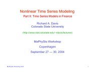
Figure 1: A longitudinal observational dataset with three patients, three distinct
drugs (A, B, and C) and two distinct outcome events (X and O)
Figure 1 provides a schematic of LOD data for coverage periods for three
patients. Patient 1 was exposed to drug A during two separate exposure periods.
While on drug A, patient 1 experienced outcome event X on three
different occasions. Patient 2 was exposed to drugs A, B, and C during successive
non-overlapping eras. Patient 2 experienced outcome event X before
consuming any drugs and also experienced outcome event X while consuming
drug C. Patient 3 was exposed to drug C and later starting taking drug B in
addition to drug C. This patient experienced outcome event O while taking
both B and C and later experienced outcome events O and X after the drug B
and C eras had ended. We note that LODs generally provide drug prescription
dates so that construction of drug “eras” involves subtle decisions concerning
gaps between successive prescriptions as well as off-drug risk periods. With
outcome events, we think of outcomes as occurring at points in time whereas
in truth outcomes are processes spread out in time.
The methodological challenge is to estimate the strength of the association
between each drug and each outcome event, while appropriately accounting
for covariates such as other drugs and outcome events, patient demographics,
etc.
In this context, several papers have looked at vaccine safety, for example,
Lieu et al. (2007), McClure et al. (2008), and Walker (2009). The Vaccine

4 D. Madigan et al.
Safety Datalink provides an early example of a LOD specifically designed for
safety. Papers focusing on drug safety include Curtis et al. (2008), Jin et al.
(2008), Kulldorff et al. (2008), Li (2009), Noren et al. (2008), and Schneeweiss
et al. (2009).
3. THE SELF-CONTROLLED CASE SERIES METHOD
Farrington (1995) proposed the self-controlled case series (SCCS) method in
order to estimate the relative incidence of adverse events to assess vaccine
safety. The major features of SCCS are that (1) it automatically controls for
time-fixed covariates that don’t vary within a person during the study period,
and (2) only cases (individuals with at least one event) need to be included
in the analysis. With SCCS, each individual serves as their own control. In
other words, SCCS compares outcome event rates during times when a person
is exposed versus outcome event rates during times when the same person is
unexposed. In effect, the cases’ unexposed time lets us infer expectations
about what would have happened during their exposed time had they not
been exposed.
SCCS is one of several self-controlled methods that the epidemiology literature
describes, many of which are variants on the case-crossover method
(Maclure, 1991). However unlike the case-crossover method, which typically
requires the choice of a comparator time period to serve as a control, SCCS
makes use of all available temporal information without the need for selection.
Epidemiological applications of SCCS tend to focus on situations with
small sample sizes and few exposure variables of interest. In contrast, the
problem of drug safety surveillance in LODs must contend with millions of
individuals and millions of potential drug exposures. The size of the problem
presents a major computational challenge – ensuring the availability of an
efficient optimization procedure is essential for a feasible implementation.
3.1. One drug, one adverse event
We will first focus on the case where there is one drug (e.g. Vioxx) and one
adverse event (e.g. myocardial infarction, MI) of interest.
To set up the notation, i will index individuals from 1 to N. Events and
exposures in our databases are recorded with dates, so temporal information
is available down to the level of days (indexed by d). Let τ i be the number of
days that person i is observed, with (i,d) being their dth day of observation.
The number of events on day (i,d) is denoted by y id , and drug exposure is
indicated by x id , where x id = 1 if i is exposed to the drug on (i,d), and 0
otherwise.
SCCS assumes that AEs arise according to a non-homogeneous Poisson
process, where the underlying event rate is modulated by drug exposure. We

Self-Controlled Case Series 5
will start with the simple assumption that person i has their own individual
baseline event rate e φi , which is constant over time. Under the SCCS model,
drug exposure yields a multiplicative effect of e β on the baseline incidence
rate. In other words, the event intensity for person i on day d can be written
as a function of drug exposure x id .
λ id = e φi+βx id
The number of events observed on (i,d) given the current exposure status is
distributed as a Poisson random variable with rate λ id , which has the following
density:
P (y id | x id ) = e−λ id
λ y id
id
y id !
The SCCS likelihood contribution for person i is the joint probability of
the observed sequence of events, conditional on the observed exposures
∏τ i
L c i = P (y i1 , . . . , y iτi | x i1 , . . . , x iτi ) = P (y i | x i ) = P (y id | x id )
There are two assumptions implicit in the Poisson model that allow us to
write out this likelihood:
d=1
(i) events are conditionally independent given exposures
y id ⊥ y id ′ | x i for d ≠ d ′ , and
(ii) past events are conditionally independent of future exposures given the
current exposure
y id ⊥ x id ′ | x id for d ≠ d ′ .
These assumptions are likely to be violated in practice (e.g., one might
expect that having an MI increase the future risk of an MI and also impacts
future drug usage), however they allow for simplifications in the model.
At this point one could maximixe the full log-likelihood over all individuals
(l c = ∑ i log Lc i ) in order to estimate the parameters. However since our primary
goal is to assess drug safety, the drug effect β is of primary interest and
the person-specific φ i effects are nuisance parameters. A further complication
is that claims databases can contain well over 10 million patients. Since the dimension
of the vector of person-specific parameters φ = (φ 1 , . . . , φ N ) ′ is equal
to the number of individuals N, estimation of φ would call for optimization
in an ultra high-dimensional space and presumably would be computationally
prohibitive.

6 D. Madigan et al.
In order to avoid estimating the nuisance parameter, we can condition on
its sufficient statistic and remove the dependence on φ i . Under the Poisson
model this sufficient statistic is the total number of events person i has over
their entire observation period, which we denote by n i = ∑ d y id. For a
non-homogeneous Poisson process, n i is a Poisson random variable with rate
parameter equal to the cumulative intensity over the observation period:
∑τ i
∑τ i
n i | x i ∼ Poisson( λ id = e φi
e βx id
)
d=1
In our case the cumulative intensity is a sum (rather than an integral)
since we assume a constant intensity over each day. Conditioning on n i yields
the following likelihood for person i:
L c i = P ( y i | x i , n i ) = P ( y τ
i | x i )
i
P ( n i | x i ) ∝ ∏
d=1
d=1
( e
βx id
) yid
∑
d e βx ′ id ′
Notice that because n i is sufficient, the individual likelihood in the above
expression no longer contains φ i . This conditional likelihood takes the form
of a multinomial, but differs from a typical multinomial regression. Here
the number of “bins” (observed days) varies by person, the β parameter is
constant across days, and the covariates x id vary by day.
Assuming that patients are independent, the full conditional likelihood is
simply the product of the individual likelihoods.
L c ∝
N∏ ∏τ i
i=1 d=1
( e
βx id
) yid
∑
d e βx ′ id ′
Estimation of the drug effect can now proceed by maximizing the conditional
log-likelihood to obtain ˆβ CMLE . Winkelmann (2008) showed that this
estimator is consistent and asymptotically Normal in the Poisson case.
It is clear from the expresson for the likelihood that if person i has no
observed events (y i = 0), they will have a contribution of L c i = 1. Consequently,
person i has no effect on the estimation, and it follows that only cases
(n i ≥ 1) need to be included in the analysis.
SCCS does a within-person comparison of the event rate during exposure
to the event rate while unexposed, and thus the method is “self-controlled”.
Intuitively it follows that if i has no events, they cannot provide any information
about the relative rate at which they have events. That the SCCS
analysis relies solely on data from cases is a substantial computational advantage
– since the incidence rate of most AEs is relatively low, typical SCCS
analyses will utilize only a modest fraction of the total number of patients .

Self-Controlled Case Series 7
3.2. Multiple drug exposures and drug interactions
So far we have discussed the scenario where there is one AE and one drug
of interest. However patients generally take multiple drugs throughout the
course of their observation period. Additionally, patients may take many
different drugs at the same time point, which leads to a potential for drug
interaction effects. In order to account for the presence of multiple drugs and
interactions, the intensity expression for the SCCS model can be extended in
a natural way.
Suppose that there are p different drugs of interest, each with a corresponding
exposure indicator x idj = 1 if exposed to drug j on day (i,d); 0
otherwise. Let e βj be the multiplicative effect of drug j on the event rate.
A multiplicative model describes the intensity for patient i on day d:
λ id = e φi+β′ x id
= e φi + β1 x id1 + ··· + β p x idp
where x id = (x id1 , . . . , x idp ) ′ and β = (β 1 , . . . , β p ) ′ .
Since n i is still sufficient for φ i , person-specific effects will once again drop
out of the likelihood upon conditioning. One can derive the expression in a
similar manner to the previous case of one AE and one drug case, resulting
in:
⎡ ⎤
(
)
τ yid i
x
∏
′
L c e β′ x id
i1
i = P ( y i | n i , X i ) ∝ ∑
⎢ ⎥
d=1 d e where X ′ β′ x id ′
i = ⎣ . ⎦
x ′ iτ i
To simplify the summation in the denominator, days with the same drug
exposures can be grouped together. Suppose that there are K i distinct combinations
of drug exposures for person i. Each combination of exposures defines
an exposure group, indexed by k = 1, . . . , K i .
For person i and exposure group k, we need to know the number of events i
has while exposed to k (y ik ) along with the length of time i spends in k (l ik ).
For person i we only require information for each of K i exposure groups,
rather than for all τ i days. This allows for coarser data and more efficient
storage – since patients tend to take drugs over extended periods of time, K i
is typically much smaller than τ i .
L c
∝
N∏
∏K i
i=1 k=1
(
e β′ x ik
∑
k ′ l ik ′e β′ x ik ′
) yik
(1)
SCCS can be further extended to include interactions and time-varying
covariates (e.g. age groups). The intensity on (i,d) including two-way drug

8 D. Madigan et al.
interactions and a vector of time-varying covariates z id can be written as
λ id = e φi + β′ x id + ∑ r≠s γrs x idr x ids + α ′ z id
where γ denotes a two-way interaction between drugs r and s.
Remark 1. In practice, many adverse effects can occur at most once in
a given day suggesting a binary rather than Poisson model. One can show
that adopting a logistic model yields an identical conditional likelihood to (1).
This equivalence allows shifting to a logistic model with follow-up truncated
at the outcome event, when that event is the onset of an enduring condition
that permanently changes exposure propensity (see Discussion below.)
Remark 2. It is straightforward to show that the conditional likelihood
in (1) is log-concave.
3.3. Bayesian Self-Controlled Case Series
We have now set up the full conditional likelihood for multiple drugs, so one
could proceed by finding conditional maximum likelihood estimates of the
drug parameter vector β. However in the problem of drug safety surveillance
in LODs there are millions of potential drug exposure predictors (tens
of thousands of drug main effects along with drug interactions). This high
dimensionality leads to potential overfitting under the usual maximum likelihood
approach, so regularization is necessary.
We take a Bayesian approach by putting a prior over the drug effect parameter
vector and performing inference based on posterior mode estimates.
There are many choices of prior distributions that shrink the parameter estimates
toward zero and address overfitting. In particular, we focus on the (1)
Normal prior and (2) Laplacian prior.
(i) Normal prior. Here we shrink the estimates toward zero by putting an
independent Normal prior on each of the parameter components. Taking
the posterior mode estimates would be analogous to a ridge Poisson
regression, placing a constraint on the L 2 -norm of the parameter vector.
(ii) Laplace prior. Under this choice of prior a portion of the posterior
mode estimates will shrink all the way to zero, and their corresponding
predictors will effectively be selected out of the model. This is equivalent
to a lasso Poisson regression, where there is a constraint on the L 1 -norm
of the parameter vector estimate.
Efficient algorithms exist for finding posterior modes, rendering our approach
tractable even in the large-scale setting. In particular, we have adapted
the cyclic-coordinate descent algorithm of Genkin et al. (2007) to the SCCS
context. An open-source implementation is available at http://omop.fnih.org.

Self-Controlled Case Series 9
4. EXTENSIONS TO THE BASIC SCCS MODEL
4.1. Relaxing the Independence Assumptions I: Events
.
Farrington and Hocine (2010) present an approach that extends SCCS to
allow for within-individual event dependence. This method treats the vector
of observed event times t i = (t i1 , . . . , t ini ) ′ for each individual i as a single
point in an n i -dimensional region, where n i denotes the number of events
experienced by individual i. This region is restricted to Q i (n i ) = {t i ∈
(a i , b i ] ni : t i1 < · · · < t ini } (where (a i , b i ] denotes the observation period for
individual i) since the components of t i are ordered by time, and no event
times can occur outside of the observation window (a i , b i ]. Standard SCCS
assumes that events are realizations of a one-dimensional Poisson process
and conditions upon the observed number of events n i . Under Farrington
and Hocine’s model, however, the event time vector t i is treated as a single
point arising from an n i -dimensional Poisson process. In this framework,
conditioning on n i is equivalent to conditioning on the occurrence of a single
point in the region Q i (n i ).
If λ i (t 1 , . . . , t ni | x i ) is the intensity of the n i -dimensional Poisson process
on Q i (n i ), the conditional likelihood of t i given the occurrence of one such
point in Q i (n i ) is
L ni
i =
∫
Q i(n i)
λ i (t i1 , . . . , t ini | x i )
(2)
λ i (u 1 , . . . , u ni | x i )du 1 · · · du ni
Farrington and Hocine assume that the n i -dimensional Poisson intensity
can be written in the form
∏n i
λ i (t 1 , . . . , t ni | x i ) = λ i (t j | x i ) × H ni (t 1 , . . . , t ni ) (3)
j=1
where the product term is made up of independent univariate intensities
λ i (t | x i ), and the H ni (.) function determines the dependence between events.
From (2) and (3) we can see that terms of λ i (t | x i ) that are fixed in time
will cancel out of the conditional likelihood, as they do in the original SCCS
model. Similarly, fixed terms of H ni (.) will also drop out of the conditional
likelihood. Farrington and Hoccine explore different possible choices for H.
4.2. Relaxing the Independence Assumptions II: The PD Model
.
The PD-SCCS model (Simpson, 2011) extends SCCS to allow positive
dependence between events, meaning that the occurrence of an event can

10 D. Madigan et al.
increase an individual’s future event risk. Let N i (t) record the number of
events that person i has experienced up until time t. Assume, as before, that
i has n i total events during their observation period and that these events
occur at times t i1 < · · · < t ini . It is convenient to define a counting process,
such as N i (t), in terms of its intensity function λ i (t | x i (t)). This function
gives the instantaneous probability that an event occurs at time t, given the
history of the process and covariates. Under the SCCS model, the Poisson
intensity for i at time t is
λ i (t | x i (t)) = e φi+β′ x i(t)
(4)
as was previously described. PD-SCCS extends this model by incorporating
N i (t − ), the number of events that i has experienced up to but not including
time t, as an additive effect on the individual baseline e φi . The PD-SCCS
intensity function takes the form
λ i (t | x i (t)) = (e φi + δN i (t − )) e β′ x i(t)
(5)
where δ is the parameter that controls the level of dependence between events.
Based on plugging the PD-SCCS intensity (5) into the likelihood expression
for a general intensity-based process, one can see that the total number of
events n i is sufficient for the nuisance parameter φ i . As in the SCCS model,
conditioning on n i removes φ i from the likelihood expression. Symmetry
arguments yield a closed form for the conditional likelihood, which in the denominator
requires integrating over all possible ways for i to have n i events
during their observation period. Inference for β and δ is based on this conditional
likelihood. Since the intensity function must be non-negative, the
event dependence parameter is restricted to δ > 0. In the case that δ = 0, the
PD-SCCS intensity model in (5) reduces to that of the SCCS model in (4).
4.3. Relaxing the Independence Assumptions III: Exposures
.
As discussed above, the SCCS model assumes that events are conditionally
independent of subsequent exposures. Farrington et al. (2009) present
an ingenious relaxation of this assumption using a counterfactual modeling
approach. Their approach applies to the specific situation where the risk
returns to its baseline level at the end of each risk period, where the event
of interest is non-recurrent, and where the occurence of the event precludes
future exposures.
Here we sketch the Farrington et al. approach using a simplified version of
their running example. Consider a situation in which each individual can have
up to two exposures. For individual i, again denote by (a i , b i ] the observation
period and denote by c i1 and c i2 the actual exposure times, should they occur.

Self-Controlled Case Series 11
For notational simplicity, we consider point exposures followed by some
known increased-risk time. The exposures then partition the observation
period into up to five periods indexed by j: a control period, followed by
an increased-risk period, followed by a control period, followed by a second
increased-risk period, followed by a final control period. Denote by n ij the
number of events occurring in the jth period, n ij ∈ {0, 1}. Let β 1 and β 2 denote
the log relative incidences associated with the first and second increased
risk periods respectively and denote by T i the event time.
If T i occurs after c i2 then no further exposures can occur and inference
about β 2 can proceed in the usual fashion. Inference for β 1 is more complex
in the situation where the event occurs after just one exposure becuase the
timing of the counterfactual second exposure is then unavailable. Farrington
et al. then make the following key observation: suppose, counterfactually,
that no individual experienced a second exposure. Then it would be possible
to estimate β 1 without bias. For this to work, we would need to know n ∗ i4 ,
the number of events in the fourth period, had no second exposure occurred.
This is missing for those individuals that did in fact have a second exposure.
However, n i4 e −β2 is an unbiased estimate of n ∗ i4 for these individuals - this
amounts to backing out the actual elevated risk during the second exposure.
Using n ∗ i4 in place of n i4 then leads to an unbiased estimate of β 1 .
Farrington et al. present the general case, an associated sandwich estimator
for the variance, and also a computationally efficient equivalent approach
based on pseudo likelihood.
We note that Roy et al. (2006) present an alternative approach.
4.4. Structured SCCS Models
. We are currently exploring several extensions to the basic model.
(i) Hierarchical model: Drugs. Drugs form drug classes. For example,
Vioxx is a Cox-2 inhibitor. Cox-2 inhibitors in turn are non-steroidal
anti-inflammatories. A natural extension assumes regression coefficients
for drugs from within a single class arise exchangeably from a common
prior distribution. This hierarchy could extend to multiple levels.
(ii) Hierarchical model: AEs. AEs also form AE classes. For example, an
MI is a cardiovascular thrombotic (CVT) event, a class that includes, for
example, ischemic stroke and unstable angina. In turn, CVT events belong
to a broader class of cardiovascular events. This extension assumes
that the regression coefficients for a particular drug but for different
AEs within a class arise from a common prior distribution. Again this
hierarchy could extend to multiple levels.

12 D. Madigan et al.
5. DISCUSSION
We have described self-controlled case series methods for post-approval drug
safety risk estimation, some Bayesian and some not. Key advantages of the
self-controlled case series approach include:
• SCCS adjusts for all time-invariant multiplicative confounders,
• Estimation requires only cases, and
• A regularized/Bayesian implementation of SCCS scales to large databases
with the potential to adjust for large numbers of time-varying covariates.
The main problems with the SCCS approach concern the underlying independence
assumptions, in particular, the assumption that events are conditionally
independent, and the assumption that the exposure distribution and
the observation period must be independent of event times. We described
approaches to circumvent these assumptions and these may be useful in some
applications.
Furthermore, since SCCS estimates the exposure-outcome association in
cases, it ignores data on individuals in the study population that did not experience
the outcome event. For example, there may be seasonality driving both
the exposure and the outcome, where season is an important time-varying covariate.
To adjust for seasonality, it is helpful to address both (a) the relation
between season and the exposure, and (b) the relation between season and
the outcome. While SCCS can incorporate time varying covariates, ignoring
Sentinel’s rich data on the non-cases limits our power to address (a). In another
paper in this issue, we discuss how analyses of data from non-cases can
supplement case-based analyses
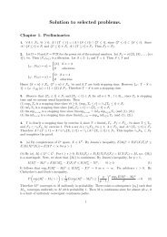
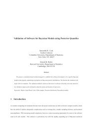
We note that one possible approach to dealing with the exposure independence
issue is to truncate observation time after the first event occurrence.
This violates other SCCS assumptions but may still be useful in practice. Figure
2 shows estimates for a number of drug-outcome pairs with and without
truncation. Clearly the truncation does alter some estimated relative risks
substantially and future work will evaluate the empirical performance of this
approach.
Real-life LODs are noisy and have the potential to introduce all sorts
of artifacts and biases into analyses. For example, conditions and the drugs
prescribed to treat the conditions are often recorded simultaneously at a single
visit to the doctor, even though the condition actually predated the visit. This
can introduce “confounding by indication” - the drug used to treat a condition
can appear to be caused by the condition. Many such challenges exist and it
remains to be seen whether or not false positives will render risk identification
in LODs impractical.

Self-Controlled Case Series 13
Since all methods rely on dubious assumptions, future research will focus
on establishing the operating characteristics of competing approaches. The
Observational Medical Outcomes Partnership (OMOP) has empirically compared
the predictive performance of SCCS, multivariate SCCS, and a wide variety
of competing methods. Initial results suggest that SCCS is competitive
with other methods and multivariate SCCS is a top performer. Nonetheless,
the performance of all methods in OMOP leaves much room for improvement.
REFERENCES
Curtis, J. R., Cheng, H., Delzell, E., Fram, D., Kilgore, M., Saag, K., Yun,
H., and DuMouchel, W. (2008). Adaptation of Bayesian data mining
algorithms to longitudinal claims data. Medical Care, 46, 969-975.
Farrington, P. (1995). Relative incidence estimation from case series for
vaccine safety evaluation. Biometrics 51, 228–235.
Farrington, C. P., Whitaker, H. J. and Hocine, M. N. (2009). Case series
analysis for censored, perturbed or curtailed post-event exposures.
Biostatistics, 10, 3–16.
Farrington, P. and Hocine, M.N. (2010). Within-individual dependence in
self-controlled case series models for recurrent events. Appl. Statist. 59,
457–475.
Genkin, A., Lewis, D. D., and Madigan, D. (2007) Large-scale Bayesian
logistic regression for text categorization,Technometrics 49, 291–304.
Jin, H., Chen, J., He, H., Williams, G.J., Kelman, C., and OḰeefe, C.M.
(2008). Mining unexpected temporal associations: Applications in
detecting adverse drug reactions. IEEE Transactions on Information
Technology in Biomedicine, 12, 488–500.
Kulldorff, M., Davis, R.L., Kolczak, M., Lewis, E., Lieu, T., and Platt, R.
(2008). A maximized sequential probability ratio test for drug and
vaccine safety surveillance. Preprint.
Li, L. (2009). A conditional sequential sampling procedure for drug safety
surveillance. Statistics in Medicine. DOI:10.1002/sim.3689
Lieu, T.A., Kulldorff, M., Davis, R.L., Lewis, E.M., Weintraub, E., Yih, K.,
Yin, R., Brown, J.S., and Platt, R. (2007). Real-time vaccine safety
surveillance for the early detection of adverse events. Medical Care, 45,
S89–95.
Maclure, M. (1991). The Case-Crossover Design: A Method for Studying
Transient Effects on the Risk of Acute Events. American Journal of
Epidemiology, 133, 144–153.
McClure, D. L., Glanz, J. M., Xu, S., Hambidge, S. J., Mullooly, J. P., and
Baggs, J. (2008). Comparison of epidemiologic methods for active
surveillance of vaccine safety. Vaccine, doi:10:1016/j.vaccine.2008.03.074.

14 D. Madigan et al.
Noren, G. N., Bate, A., Hopstadius, J., Star, K., and Edwards, I. R. (2008).
Temporal pattern discovery for trends and transient effects: its
application to patient records. In: Proceedings of the Fourteenth
International Conference on Knowledge Discovery and Data Mining
SIGKDD 2008, 963–971.
Roy, J., Alderson, D., Hogan, J.W., and Tashima, K. T. (2006). Conditional
inference methods for incomplete Poisson data with endogenous
time-varying covariates, J. Amer. Statist. Assoc. 101, 424–434.
Schneeweiss, S., Rassen, J. A., Glynn, R. J., Avorn, J., Mogun, H., and
Brookhart, M. A. (2009). High-dimensional propensity scoring
adjustment in studies of treatment effects using health care claims data.
Epidemiology, 20, 512-522.
Simpson, S.E. (2011). The positive-dependence self-controlled case series
model. Submitted.
Walker, A. M. (2009). Signal detection for vaccine side effects that have not
been specified in advance. Preprint.
Winkelmann, R. (2008). Econometric Analysis of Count Data. Springer.

Self-Controlled Case Series 15
Truncated versus Non−Truncated SCCS, log RR
Truncated
−0.4 −0.2 0.0 0.2 0.4 0.6
●
●
true positives
negative controls
Typical Aplastic ●
● Typical Acute Re
Warfarin Hip Frac ●
● Typical Upper GI
●
Tricycli Angioede
●
●
Antibiot Acute Li ●
Typical Acute my
Typical Bleeding
Beta blo Acute my
Antibiot Acute Re
●
●
● Antiepil Aplastic
●
Antibiot Aplastic
●
Warfarin Aplastic
Antibiot Angioede
●
●
Bisphosp Mortalit
●
●
Benzodia Typical Angioede Antibiot Hip Tricycli Frac Acute Upper myGI
Typical Acute Li Tricycli Mortalit Beta blo Mortalit
● ●
●
●
Beta ●
blo Angioede
● ACE Inhi Aplastic
●
●
●
●
●
Amphoter Acute
Amphoter
Li
Upper Warfarin GI Benzodia Acute myMortalit
● Bisphosp Aplastic
Benzodia Acute ● my
Benzodia Bleeding Antiepil Acute Re
●
● Typical Mortalit ● Benzodia Acute Li
Antibiot Bleeding ●
Beta blo Acute Re
Antibiot Upper GI ●
Beta Typical blo Aplastic Angioede ● ●
●
Amphoter Aplastic ●
● ●
●
Warfarin Angioede
Amphoter
● Benzodia
Acute
Upper
ReWarfarin GI
Upper GI
Amphoter Acute my ● ● Antibiot Mortalit
Warfarin Acute Li
●
●
●
Tricycli AplasticAntiepil Mortalit
Beta blo Acute Li
● Tricycli Acute Li ●
● Tricycli Acute my
Amphoter Warfarin BleedingAcute ● Re ● Antiepil Hip Frac ●
●
●
● Tricycli Bleeding Beta blo Upper GI
Antibiot Hip Frac
●
Benzodia Aplastic ●
ACE Inhi Acute Li Bisphosp Acute Li
●Tricycli Benzodia Hip Frac Acute Re
●
Tricycli Acute Re
●
Warfarin Mortalit ●
●
●
● ACE Inhi Upper GI
●
Beta blo Hip Frac
●
Antiepil Angioede ACE Inhi ● Bleeding
Beta blo Bleeding ●
●
ACE Inhi Acute Re Bisphosp ● Acute my
●
Antiepil Acute Li
Bisphosp Hip Frac ●
Bisphosp Acute Re
● Benzodia Hip Frac
●
Bisphosp Angioede
ACE Inhi ● Antiepil Acute my Bleeding ●
Antiepil Upper GI ●
●
Bisphosp Upper GI
● ACE Inhi Hip Frac
●
●
ACE Inhi Mortalit
Bisphosp Bleeding
●
Warfarin Bleeding
●
ACE Inhi Angioede
●
Antiepil Acute my
−0.2 0.0 0.2 0.4 0.6 0.8 1.0
NotTruncated
MSCCSv1.0_MSLR_ctype_2_prior_normal_var_0.1_swindo_n30_ds_1_
Figure 2: Relative risk estimates from SCCS versus truncated SCCS for 53
drug-outcome pairs in the OMOP experiment.