The Self-Controlled Case Series - Department of Statistics ...

6 D. Madigan et al.
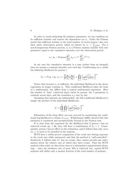
In order to avoid estimating the nuisance parameter, we can condition on
its sufficient statistic and remove the dependence on φ i . Under the Poisson
model this sufficient statistic is the total number of events person i has over
their entire observation period, which we denote by n i = ∑ d y id. For a
non-homogeneous Poisson process, n i is a Poisson random variable with rate
parameter equal to the cumulative intensity over the observation period:
∑τ i
∑τ i
n i | x i ∼ Poisson( λ id = e φi
e βx id
)
d=1
In our case the cumulative intensity is a sum (rather than an integral)
since we assume a constant intensity over each day. Conditioning on n i yields
the following likelihood for person i:
L c i = P ( y i | x i , n i ) = P ( y τ
i | x i )
i
P ( n i | x i ) ∝ ∏
d=1
d=1
( e
βx id
) yid
∑
d e βx ′ id ′
Notice that because n i is sufficient, the individual likelihood in the above
expression no longer contains φ i . This conditional likelihood takes the form
of a multinomial, but differs from a typical multinomial regression. Here
the number of “bins” (observed days) varies by person, the β parameter is
constant across days, and the covariates x id vary by day.
Assuming that patients are independent, the full conditional likelihood is
simply the product of the individual likelihoods.
L c ∝
N∏ ∏τ i
i=1 d=1
( e
βx id
) yid
∑
d e βx ′ id ′
Estimation of the drug effect can now proceed by maximizing the conditional
log-likelihood to obtain ˆβ CMLE . Winkelmann (2008) showed that this
estimator is consistent and asymptotically Normal in the Poisson case.
It is clear from the expresson for the likelihood that if person i has no
observed events (y i = 0), they will have a contribution of L c i = 1. Consequently,
person i has no effect on the estimation, and it follows that only cases
(n i ≥ 1) need to be included in the analysis.
SCCS does a within-person comparison of the event rate during exposure
to the event rate while unexposed, and thus the method is “self-controlled”.
Intuitively it follows that if i has no events, they cannot provide any information
about the relative rate at which they have events. That the SCCS
analysis relies solely on data from cases is a substantial computational advantage
– since the incidence rate of most AEs is relatively low, typical SCCS
analyses will utilize only a modest fraction of the total number of patients .