The Self-Controlled Case Series - Department of Statistics ...
The Self-Controlled Case Series - Department of Statistics ...
The Self-Controlled Case Series - Department of Statistics ...

Create successful ePaper yourself
Turn your PDF publications into a flip-book with our unique Google optimized e-Paper software.
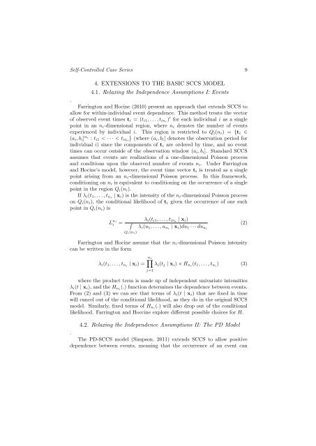
<strong>Self</strong>-<strong>Controlled</strong> <strong>Case</strong> <strong>Series</strong> 9<br />
4. EXTENSIONS TO THE BASIC SCCS MODEL<br />
4.1. Relaxing the Independence Assumptions I: Events<br />
.<br />
Farrington and Hocine (2010) present an approach that extends SCCS to<br />
allow for within-individual event dependence. This method treats the vector<br />
<strong>of</strong> observed event times t i = (t i1 , . . . , t ini ) ′ for each individual i as a single<br />
point in an n i -dimensional region, where n i denotes the number <strong>of</strong> events<br />
experienced by individual i. This region is restricted to Q i (n i ) = {t i ∈<br />
(a i , b i ] ni : t i1 < · · · < t ini } (where (a i , b i ] denotes the observation period for<br />
individual i) since the components <strong>of</strong> t i are ordered by time, and no event<br />
times can occur outside <strong>of</strong> the observation window (a i , b i ]. Standard SCCS<br />
assumes that events are realizations <strong>of</strong> a one-dimensional Poisson process<br />
and conditions upon the observed number <strong>of</strong> events n i . Under Farrington<br />
and Hocine’s model, however, the event time vector t i is treated as a single<br />
point arising from an n i -dimensional Poisson process. In this framework,<br />
conditioning on n i is equivalent to conditioning on the occurrence <strong>of</strong> a single<br />
point in the region Q i (n i ).<br />
If λ i (t 1 , . . . , t ni | x i ) is the intensity <strong>of</strong> the n i -dimensional Poisson process<br />
on Q i (n i ), the conditional likelihood <strong>of</strong> t i given the occurrence <strong>of</strong> one such<br />
point in Q i (n i ) is<br />
L ni<br />
i =<br />
∫<br />
Q i(n i)<br />
λ i (t i1 , . . . , t ini | x i )<br />
(2)<br />
λ i (u 1 , . . . , u ni | x i )du 1 · · · du ni<br />
Farrington and Hocine assume that the n i -dimensional Poisson intensity<br />
can be written in the form<br />
∏n i<br />
λ i (t 1 , . . . , t ni | x i ) = λ i (t j | x i ) × H ni (t 1 , . . . , t ni ) (3)<br />
j=1<br />
where the product term is made up <strong>of</strong> independent univariate intensities<br />
λ i (t | x i ), and the H ni (.) function determines the dependence between events.<br />
From (2) and (3) we can see that terms <strong>of</strong> λ i (t | x i ) that are fixed in time<br />
will cancel out <strong>of</strong> the conditional likelihood, as they do in the original SCCS<br />
model. Similarly, fixed terms <strong>of</strong> H ni (.) will also drop out <strong>of</strong> the conditional<br />
likelihood. Farrington and Hoccine explore different possible choices for H.<br />
4.2. Relaxing the Independence Assumptions II: <strong>The</strong> PD Model<br />
.<br />
<strong>The</strong> PD-SCCS model (Simpson, 2011) extends SCCS to allow positive<br />
dependence between events, meaning that the occurrence <strong>of</strong> an event can