Companion notes - The Department of Statistics and Applied ...

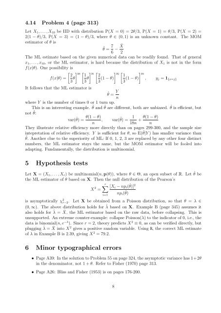
4.14 Problem 4 (page 313)
Let X 1 , . . . , X 10 be IID with distribution P(X = 0) = 2θ/3, P(X = 1) = θ/3, P(X = 2) =
2(1 − θ)/3, P(X = 3) = (1 − θ)/3, where θ ∈ (0, 1) is an unknown constant. The MOM
estimator of θ is
˜θ = 7 6 − ¯X
2
The ML estimate based on the given numerical data can be readily found. That of general
x 1 , . . . , x 10 , or the ML estimator, is hard because the distribution of X 1 is not in the form
f(x|θ). One possibility is
[ ] y0
[ ] y1
[ ] y2
[ ] y3
2 1 2 1
f(x|θ) =
3 θ 3 θ 3 (1 − θ) 3 (1 − θ) , y j = 1 {x=j}
It follows that the ML estimator is
ˆθ = Y n
where Y is the number of times 0 or 1 turn up.
This is an interesting example. ˜θ and ˆθ are different, both are unbiased. ˆθ is efficient, but
not ˜θ:
θ(1 − θ)
var(ˆθ) = , var(˜θ) = 1 θ(1 − θ)
+
n
18n n
They illustrate relative efficiency more directly than on pages 299-300, and the sample size
intepretation of relative efficiency. Y is sufficient for θ, so E(˜θ|Y ) has smaller variance than
˜θ. Another clue to the superiority of ML: If 0, 1, 2, 3 are replaced by any other four distinct
numbers, the ML estimator stays the same, but the MOM estimator will be fooled into
adapting. Fundamentally, the distribution is multinomial.
5 Hypothesis tests
Let X = (X 1 , . . . , X r ) be multinomial(n, p(θ)), where θ ∈ Θ, an open subset of R. Let ˆθ be
the ML estimator of θ based on X. Then the null distribution of the Pearson’s
r∑
X 2 [X i − np i (ˆθ)] 2
=
np i (ˆθ)
i=1
is asymptotically χ 2 r−2. Let X be obtained from a Poisson distribution, so that θ = λ ∈
(0, ∞). The above distribution holds for ˆλ based on X. Example B (page 345) assumes it
also holds for ˆλ = ¯X, the ML estimator based on the raw data, before collapsing. This is
unsupported. An extreme counter-example: collapse Poisson(λ) to the indicator of 0, i.e., the
data is binomial(n, e −λ ). Since r = 2, theory predicts X 2 ≡ 0, as can be verified directly, but
plugging ˆλ = ¯X into X 2 gives a positive random variable. Using R, the correct ML estimate
of λ in Example B is 2.39, giving X 2 = 79.2.
6 Minor typographical errors
• Page A39: In the solution to Problem 55 on page 324, the asymptotic variance has 1+2θ
in the denominator, not 1 + θ. Refer to Fisher (1970) page 313.
• Page A26: Bliss and Fisher (1953) is on pages 176-200.
8