ST4241: Design and Analysis of Clinical Trials - The Department of ...
ST4241: Design and Analysis of Clinical Trials - The Department of ...
ST4241: Design and Analysis of Clinical Trials - The Department of ...

You also want an ePaper? Increase the reach of your titles
YUMPU automatically turns print PDFs into web optimized ePapers that Google loves.
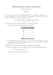
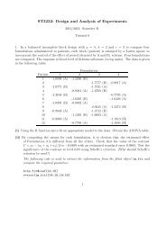
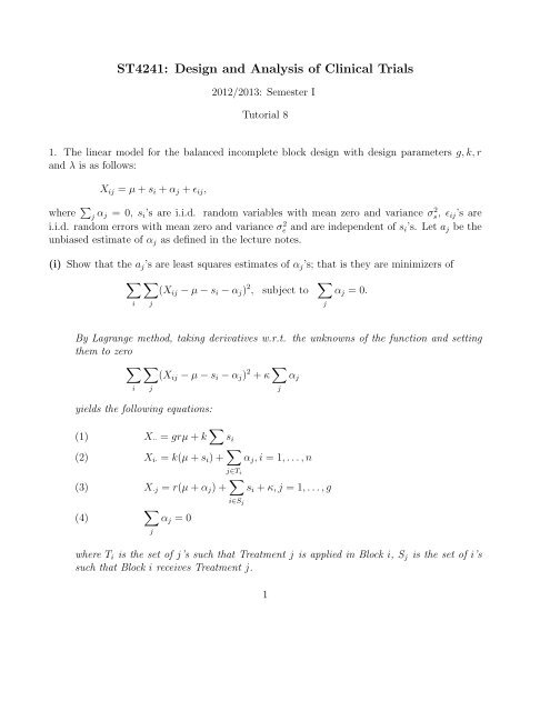
<strong>ST4241</strong>: <strong>Design</strong> <strong>and</strong> <strong>Analysis</strong> <strong>of</strong> <strong>Clinical</strong> <strong>Trials</strong><br />
2012/2013: Semester I<br />
Tutorial 8<br />
1. <strong>The</strong> linear model for the balanced incomplete block design with design parameters g, k, r<br />
<strong>and</strong> λ is as follows:<br />
X ij = µ + s i + α j + ɛ ij ,<br />
where ∑ j α j = 0, s i ’s are i.i.d. r<strong>and</strong>om variables with mean zero <strong>and</strong> variance σ 2 s, ɛ ij ’s are<br />
i.i.d. r<strong>and</strong>om errors with mean zero <strong>and</strong> variance σ 2 e <strong>and</strong> are independent <strong>of</strong> s i ’s. Let a j be the<br />
unbiased estimate <strong>of</strong> α j as defined in the lecture notes.<br />
(i) Show that the a j ’s are least squares estimates <strong>of</strong> α j ’s; that is they are minimizers <strong>of</strong><br />
∑ ∑<br />
(X ij − µ − s i − α j ) 2 , subject to ∑<br />
i j<br />
j<br />
α j = 0.<br />
By Lagrange method, taking derivatives w.r.t. the unknowns <strong>of</strong> the function <strong>and</strong> setting<br />
them to zero<br />
∑ ∑<br />
(X ij − µ − s i − α j ) 2 + κ ∑ α j<br />
i j<br />
j<br />
yields the following equations:<br />
(1)<br />
(2)<br />
(3)<br />
(4)<br />
X·· = grµ + k ∑ s i<br />
X i· = k(µ + s i ) + ∑ α j , i = 1, . . . , n<br />
j∈T i<br />
X·j = r(µ + α j ) + ∑ s i + κ, j = 1, . . . , g<br />
i∈S j<br />
∑<br />
α j = 0<br />
j<br />
where T i is the set <strong>of</strong> j’s such that Treatment j is applied in Block i, S j is the set <strong>of</strong> i’s<br />
such that Block i receives Treatment j.<br />
1
Sum up (3) over j yields<br />
(5) X·· = grµ + k ∑ s i + gκ<br />
(5)-(1) yields that κ = 0. From (2) <strong>and</strong> (3), we have<br />
(6)<br />
(7)<br />
µ + s i = ¯X i· − 1 k<br />
∑<br />
j ′ ∈T i<br />
α j<br />
′<br />
X·j = rα j + ∑ i∈S j<br />
(µ + s i )<br />
Substituting (6) into (7) yields<br />
It yields<br />
(ii) Show that<br />
X·j = rα j + ∑ ( ¯X i· − 1 ∑<br />
α<br />
k j<br />
′)<br />
i∈S j j ′ ∈T i<br />
= rα j + rM j − 1 ∑ ∑<br />
k<br />
α j<br />
′<br />
i∈S j j ′ ∈T i<br />
= rα j + rM j − r − λ<br />
k α j.<br />
(1 − r − λ<br />
kr )α j = ¯X·j − M j , i.e., α j = 1<br />
eff ( ¯X·j − M j ).<br />
Var(a j ) =<br />
where eff = g(k−1)<br />
k(g−1) .<br />
σ2 e<br />
reff<br />
g − 1<br />
, Cov(a j , a k ) = − σ2 e<br />
g<br />
1<br />
reff g ,<br />
Write<br />
¯X·j − M j = 1 ∑<br />
(X ij −<br />
r<br />
¯X i·)<br />
i∈S j<br />
= 1 ∑<br />
(α j − 1 ∑<br />
α<br />
r k j<br />
′ + ɛ ij − 1 ∑<br />
ɛ<br />
k ij<br />
′).<br />
i∈S j j ′ ∈T i j ′ ∈T i<br />
2
Thus<br />
Var( ¯X·j − M j ) = 1 ∑<br />
Var(ɛ<br />
r 2 ij − 1 ∑<br />
ɛ<br />
k ij<br />
′)<br />
i∈S j j ′ ∈T i<br />
= 1 ∑<br />
[(1 − 1 r 2 k )2 + k − 1 ]σ<br />
k 2 e<br />
2<br />
i∈S j<br />
= k − 1<br />
rk σ2 e.<br />
Hence<br />
Var(a j ) = k − 1<br />
rkeff 2 σ2 e =<br />
σ2 e k − 1<br />
reff keff =<br />
σ2 e<br />
reff<br />
g − 1<br />
.<br />
g<br />
Similarly,<br />
Cov( ¯X·j − M j , ¯X·l − M l )<br />
= 1 ∑ ∑<br />
Cov(ɛ<br />
r 2 ij − 1 ∑<br />
ɛ<br />
k ij<br />
′, ɛ i ′ l − 1 ∑<br />
ɛ ′<br />
k i j<br />
′)<br />
i∈S j i ′ ∈S l j ′ ∈T i j ′ ∈T ′ i<br />
= 1 r λCov(ɛ 2 ij − 1 ∑<br />
ɛ<br />
k ij<br />
′, ɛ il − 1 ∑<br />
ɛ<br />
k ij<br />
′)<br />
j ′ ∈T i j ′ ∈T i<br />
= λ r 2 (−σ2 e<br />
k ).<br />
Hence<br />
Cov(a j , a l ) =<br />
λ<br />
r 2 eff 2 (−σ2 e<br />
k ) = − 1 σe<br />
2<br />
reff g .<br />
(iii) Show that, for any contrast ∑ g<br />
j=1 c ja j ,<br />
Var(<br />
g∑<br />
c j a j ) =<br />
j=1<br />
σ2 e<br />
reff<br />
∑<br />
c 2 j.<br />
j<br />
3
g∑<br />
Var( c j a j )<br />
j=1<br />
= ∑ j<br />
= ∑ j<br />
= ∑ j<br />
∑<br />
c j c l Cov(a j , a l )<br />
c 2 j<br />
c 2 j<br />
l<br />
σ 2<br />
reff<br />
g − 1<br />
g<br />
− ∑ j≠l<br />
σ 2<br />
reff [g − 1 + 1 g g ] = ∑ j<br />
1 σe<br />
2 c j c l<br />
reff g<br />
c 2 j<br />
σ 2<br />
reff .<br />
Note that<br />
0 = ( ∑ j<br />
c j ) 2 = ∑ j<br />
c 2 j + ∑ j≠l<br />
c j c l .<br />
2. <strong>The</strong> data from the interexaminer reliability study considered in the lecture notes is given on<br />
the next page.<br />
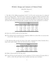
(i) Using the linear model approach, derive the F ratio for testing the significance <strong>of</strong> the<br />
differences among the examiners.<br />
Examiner<br />
Patient 1 2 3 4 5 6 Mean<br />
1 10 14 10 11.33<br />
2 3 3 1 2.33<br />
3 7 12 9 9.33<br />
4 3 8 5 5.33<br />
5 20 26 20 22.00<br />
6 20 14 20 18.00<br />
7 5 8 14 9.00<br />
8 14 18 15 15.67<br />
9 12 17 12 13.67<br />
10 18 19 13 16.67<br />
Mean 8.6 11.2 13.2 10.6 16.2 14.2 12.33<br />
<strong>The</strong> data is fitted to the following model<br />
∑10<br />
6∑<br />
X = µ 0 + s i b i + a j t j + ɛ,<br />
i=2 j=2<br />
4
where the dummy variables b i ’s <strong>and</strong> t j ’s are defined conventionally.<br />
<strong>The</strong> R code<br />
lm.fit1=lm(x~s+a)<br />
produces the following ANOVA table:<br />
Df Sum Sq Mean Sq F value Pr(>F)<br />
s 9 982.00 109.11 11.7558 2.615e-05 ***<br />
a 5 35.44 7.09 0.7638 0.5898<br />
Residuals 15 139.22 9.28<br />
<strong>The</strong> F ratio for the examiner effect is 0.7638 with a p-value 0.5898. <strong>The</strong>re is no significant<br />
effect <strong>of</strong> the examiners.<br />
(ii) By looking at the data, it seems that Examiner 5 <strong>and</strong> 6 have higher mean scores than the<br />
other examiners. One would like to see whether the following contrasts are significant:<br />
α 1 + α 2 + α 3 + α 4<br />
4<br />
α 1 + α 2 + α 3 + α 4<br />
4<br />
α 1 + α 2 + α 3 + α 4<br />
4<br />
− α 5 + α 6<br />
,<br />
2<br />
− α 5 ,<br />
− α 6 .<br />
Using an appropriate multiple comparison criterion, test the significance <strong>of</strong> the above<br />
contrasts by controlling the overall error rate at 0.05.<br />
In terms <strong>of</strong> the parameters <strong>of</strong> the linear model, the contrasts are equivalent to the linear<br />
forms:<br />
a 2 + a 3 + a 4<br />
4<br />
a 2 + a 3 + a 4<br />
4<br />
a 2 + a 3 + a 4<br />
4<br />
− a 5 + a 6<br />
,<br />
2<br />
− a 5 ,<br />
− a 6 .<br />
<strong>The</strong> estimated a j ’s <strong>and</strong> their variance matrix are as follows:<br />
5
a2 a3 a4 a5 a6<br />
1.750000 1.083333 3.333333 3.416667 1.416667<br />
a2 a3 a4 a5 a6<br />
a2 4.640741 2.320370 2.320370 2.320370 2.320370<br />
a3 2.320370 4.640741 2.320370 2.320370 2.320370<br />
a4 2.320370 2.320370 4.640741 2.320370 2.320370<br />
a5 2.320370 2.320370 2.320370 4.640741 2.320370<br />
a6 2.320370 2.320370 2.320370 2.320370 4.640741<br />
By using the above information, the test statistics for the three contrasts are computed as<br />
L 1 = −0.6633, L 2 = −1.1010, L 3 = 0.0734.<br />
<strong>The</strong> Schiffe criterion should be used. <strong>The</strong> critical value is given by √ 5F 5,15,0.05 = 3.8087.<br />
None <strong>of</strong> the contrasts is significant.<br />
3. <strong>The</strong> data form the study comparing four formulations considered in the lecture notes is given<br />
at the end <strong>of</strong> this question. Using R, fit a linear model to the data. Using the information in<br />
the fitted object, do the following:<br />
(i) By computing the means for each formulation, it is obvious form that the estimated effect<br />
<strong>of</strong> Formulation 3 is different from all the others. Check that the value <strong>of</strong> the contrast<br />
C = a 3 − (a 1 + a 2 + a 4 )/3 is −0.6489 with an estimated st<strong>and</strong>ard error 0.0883. Test the<br />
significance <strong>of</strong> the contrast at level 0.05 using Scheffe’s criterion. (Why should Scheffe’s<br />
criterion be used?)<br />
<strong>The</strong> following code is used to extract the information from the fitted object lm.fit <strong>and</strong><br />
compute the required quantities:<br />
b=lm.fit$coef[14:16]<br />
v=vcov(lm.fit)[14:16,14:16]<br />
c1 = c(-1/3,1,-1/3)<br />
t(c1)%*%b<br />
sqrt( t(c1)%*%v%*%c1 )<br />
L = t(c1)%*%b/sqrt( t(c1)%*%v%*%c1 )<br />
<strong>The</strong> computation yields the given values for C <strong>and</strong> its st<strong>and</strong>ard error. <strong>The</strong> test statistic<br />
equals −7.35599. Its absolute value, compared with √ 3F 3,8,0.05 = 3.492641, is not<br />
significant.<br />
6
(ii) Check that, <strong>of</strong> the six pairwise differences a j − a j<br />
′, only the three differences involving<br />
Formulation 3 are statistically significant by the Tukey criterion.<br />
<strong>The</strong> following code is used for the computation:<br />
c12 = c(1,0,0)<br />
c13 = c(0,1,0)<br />
c14 = c(0,0,1)<br />
c23 = c(1,-1,0)<br />
c24 = c(1,0,-1)<br />
c34 = c(0,1,-1)<br />
C = rbind(c12,c13,c14,c23,c24,c34)<br />
l = C%*%b<br />
ss = sqrt( diag( C%*%v%*%t(C)) )<br />
L = l/ss<br />
<strong>The</strong> computed test statistics corresponding the six pairs are:<br />
c12 0.76096856<br />
c13 -5.73428051<br />
c14 0.05461109<br />
c23 6.49524907<br />
c24 0.70635747<br />
c34 -5.78889161<br />
<strong>The</strong> critical value for the statistics using Tukey’s criterion is q 4,8,0.05 / √ 2 = 4.529/ √ 2 =<br />
3.2025. It is seen that c13, c23, c34 are significant.<br />
7
Formulation<br />
Patient 1 2 3 4<br />
1 -1.0894 (A) -1.3200 (B)<br />
2 -1.7577 (B) -0.9817 (A)<br />
3 -1.0771 (B) -1.7531 (A)<br />
4 -0.9381 (A) -1.6769 (B)<br />
5 -1.2044 (B) -0.7795 (A)<br />
6 -1.0395 (B) -1.0426 (A)<br />
7 -1.0991 (B) -0.8092 (A)<br />
8 -2.0245 (A) -1.3374 (B)<br />
9 -0.9846 (A) -1.4712 (B)<br />
10 -1.1395 (B) -1.6683 (A)<br />
11 -0.8069 (A) -1.1913 (B)<br />
12 -0.7789 (A) -1.1694 (B)<br />
8