CHAPTER 1: An introduction to time series and forecasting
CHAPTER 1: An introduction to time series and forecasting
CHAPTER 1: An introduction to time series and forecasting

Create successful ePaper yourself
Turn your PDF publications into a flip-book with our unique Google optimized e-Paper software.
<strong>CHAPTER</strong> 1: <strong>An</strong> <strong>introduction</strong> <strong>to</strong> <strong>time</strong> <strong>series</strong><br />
<strong>and</strong> <strong>forecasting</strong><br />
Basic Questions:<br />
1. What is a <strong>time</strong> <strong>series</strong>?<br />
2. What are the purposes of <strong>time</strong> <strong>series</strong> analysis?<br />
3. what are the difference between classical (Independent Identically Distributed (IID)) statistical<br />
analysis (e.g. inference <strong>and</strong> modelling) <strong>and</strong> <strong>time</strong> <strong>series</strong> analysis?<br />
1 Time Series<br />
A <strong>time</strong> <strong>series</strong> is a sequence of observations over <strong>time</strong>.<br />
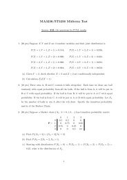
Example: Records of a person’s height:<br />
age : 1 2 3 4 5 6 7<br />
height(m) : 0.4 0.5 0.8 1.0 1.1 1.2 1.4<br />
(notation : y 1 y 2 y 3 y 4 y 5 y 6 y 7 )<br />
For this example, we have n = 7 observations. We call n the number of observations or<br />
the length of a <strong>time</strong>s <strong>series</strong>. We denote the observation at <strong>time</strong> t by y t (or x t etc.)<br />
The <strong>time</strong> <strong>series</strong> can be then denoted as<br />
{0.4, 0.5, 0.8, 1.0, 1.1, 1.2, 1.4}<br />
or<br />
{y t : t = 1, 2, ..., n}<br />
Plot of a <strong>time</strong> <strong>series</strong><br />
1
1.5<br />
height<br />
1<br />
0.5<br />
0<br />
1 2 3 4 5 6 7 8 9 10<br />
age<br />
1.5<br />
height<br />
1<br />
0.5<br />
0<br />
1 2 3 4 5 6 7 8 9 10<br />
age<br />
Figure 1:<br />
Note that the above observations are taken over equally <strong>time</strong> intervals. We can also observe<br />
the variable with unequally <strong>time</strong> intervals<br />
age : 0.5 1 1.5 2 3 5 7<br />
height(m) : 0.35 0.4 0.45 0.5 0.8 1.1 1.4<br />
Theoretically, we can observe the data continuously <strong>and</strong> get a “continuous-<strong>time</strong>” <strong>time</strong> <strong>series</strong>.<br />
Remarks: We are mainly interested in discrete-<strong>time</strong> <strong>time</strong> <strong>series</strong> with equally fixed <strong>time</strong><br />
intervals. e.g. observations made monthly, daily, weekly, etc.<br />
2
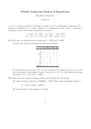
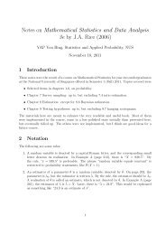
Example (Unemployment Rate (%) in Singapore)<br />
year rate year rate year rate<br />
1973 4.4 1984 2.7 1995 2.7<br />
1974 3.9 1985 4.1 1996 3.0<br />
1975 4.5 1986 6.5 1997 2.4<br />
1976 4.4 1987 4.7 1998 3.2<br />
1977 3.9 1988 3.3 1999 4.6<br />
1978 3.6 1989 2.2 2000 4.4<br />
1979 3.3 1990 1.7 2001 3.4<br />
1980 3.5 1991 1.9 2002 5.2<br />
1981 2.9 1992 2.7 2003 5.4<br />
1982 2.6 1993 2.7 2004 5.3<br />
1983 3.2 1994 2.6<br />
7<br />
6<br />
5<br />
4<br />
3<br />
2<br />
1<br />
1970 1975 1980 1985 1990 1995 2000 2005<br />
Figure 2:<br />
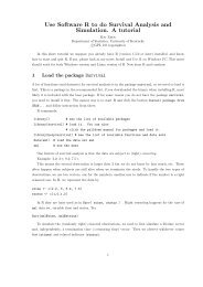
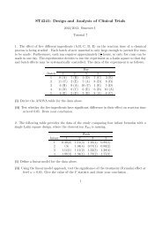
More <strong>time</strong> <strong>series</strong> [what can you observe in the <strong>time</strong> <strong>series</strong>?]<br />
7000<br />
Canadian Lynx captured (1828-1934)<br />
6000<br />
number of lynx<br />
5000<br />
4000<br />
3000<br />
2000<br />
1000<br />
0<br />
0 20 40 60 80 100 120<br />
<strong>time</strong> (year)<br />
Figure 3:<br />
3
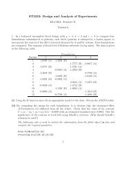
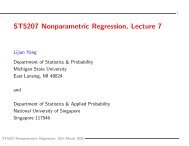
35<br />
Temperature in Hong Kong (1994-1997)<br />
daily temperature in HK<br />
30<br />
25<br />
20<br />
15<br />
10<br />
5<br />
0 200 400 600 800 1000 1200<br />
Number of patients with respira<strong>to</strong>ry problems in Hong Kong (1994)<br />
300<br />
no. of patients<br />
250<br />
200<br />
150<br />
100<br />
0 50 100 150 200 250 300 350 400<br />
<strong>time</strong> (daily)<br />
10000<br />
Measles cases in London (1944-1978)<br />
cases of measles<br />
8000<br />
6000<br />
4000<br />
2000<br />
0<br />
0 100 200 300 400 500 600 700 800 900 1000<br />
<strong>time</strong> (week)<br />
DOW s<strong>to</strong>ck index (1992-2005)<br />
15000<br />
DOW index<br />
10000<br />
5000<br />
0<br />
1992 1994 1996 1998 2000 2002 2004<br />
<strong>time</strong><br />
return: z t<br />
= log(y t<br />
) −log(y t−1<br />
)<br />
0.1<br />
0.05<br />
0<br />
−0.05<br />
−0.1<br />
1992 1994 1996 1998 2000 2002 2004<br />
<strong>time</strong><br />
4
2 Forecasting<br />
A major objective of <strong>time</strong> <strong>series</strong> analysis is <strong>forecasting</strong> of future values of the <strong>series</strong><br />
e.g. what will be the unemployment rate next year?<br />
Is there a trend in global temperature?<br />
what is the seasonal effect?<br />
what is the relationship between GDP <strong>and</strong> interest rate?<br />
Forecasting methods:<br />
1. Qualitative <strong>forecasting</strong> methods: use the opinions of experts <strong>to</strong> predict future events<br />
subjectively.<br />
2. Quantitative <strong>forecasting</strong> methods: Based the his<strong>to</strong>rical data, use statistical methods <strong>to</strong><br />
predict future values of a variable.<br />
3 The difference between the <strong>time</strong> <strong>series</strong> <strong>and</strong> IID statistics<br />
Time <strong>series</strong> data are dependent<br />
1. there is an order for the observation of <strong>time</strong> <strong>series</strong>.<br />
2. <strong>time</strong> <strong>series</strong> data are dependent. e.g. this month’s unemployment rate will be correlated<br />
with the last month’s.<br />
The problem with dependence:<br />
Consider the IID case<br />
X 1 , X 2 , · · · , X n r<strong>and</strong>om sample with mean µ <strong>and</strong> variance σ 2 . Then we estimate µ by<br />
ˆµ = (X 1 + X 2 + · · · + X n )/n<br />
5
The variance of ˆµ is<br />
we have V ar(ˆµ) → 0 as n → ∞.<br />
V ar(ˆµ) = 1 n 2 (V ar(X 1) + V ar(X 2 ) + ...V ar(X n )) = σ2<br />
n<br />
Imagine the situation where all the X i ’s are “perfectly” correlated, i.e.<br />
Cov(X i , X j ) = σ 2<br />
Corr(X i , X j ) = 1<br />
We still estimate µ by<br />
ˆµ = (X 1 + X 2 + · · · + X n )/n<br />
the variance is then<br />
V ar(ˆµ) = 1 n 2 V ar(X 1 + X 2 + · · · + X n )<br />
= 1 n∑<br />
n { V ar(X 2 i ) + 2 ∑ Cov(X i , X j )}<br />
i=1<br />
i