Use Software R to do Survival Analysis and - The Department of ...
Use Software R to do Survival Analysis and - The Department of ...
Use Software R to do Survival Analysis and - The Department of ...
Create successful ePaper yourself
Turn your PDF publications into a flip-book with our unique Google optimized e-Paper software.
<strong>Use</strong> <strong>S<strong>of</strong>tware</strong> R <strong>to</strong> <strong>do</strong> <strong>Survival</strong> <strong>Analysis</strong> <strong>and</strong><br />
Simulation. A tu<strong>to</strong>rial<br />
Mai Zhou<br />
<strong>Department</strong> <strong>of</strong> Statistics, University <strong>of</strong> Kentucky<br />
c○GPL 2.0 copyrighted<br />
In this short tu<strong>to</strong>rial we suppose you already have R (version 1.5.0 or later) installed, <strong>and</strong> know<br />
how <strong>to</strong> start <strong>and</strong> quit R. If not, please look at my notes Install <strong>and</strong> <strong>Use</strong> R on Win<strong>do</strong>ws PC. This notes<br />
should work for both Win<strong>do</strong>ws version <strong>and</strong> Linux version <strong>of</strong> R. Now start R <strong>and</strong> continue<br />
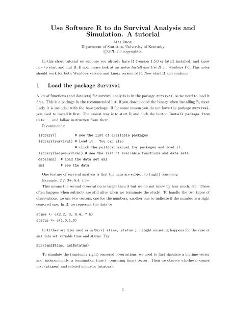
1 Load the package <strong>Survival</strong><br />
A lot <strong>of</strong> functions (<strong>and</strong> datasets) for survival analysis is in the package survival, so we need <strong>to</strong> load it<br />
first. This is a package in the recommended list, if you <strong>do</strong>wnloaded the binary when installing R, most<br />
likely it is included with the base package. If for some reason you <strong>do</strong> not have the package survival,<br />
you need <strong>to</strong> install it first. <strong>The</strong> easiest way is <strong>to</strong> start R <strong>and</strong> click the but<strong>to</strong>n Install package from<br />
CRAN... <strong>and</strong> follow instruction from there.<br />
R comm<strong>and</strong>s:<br />
library()<br />
library(survival) # load it.<br />
# see the list <strong>of</strong> available packages<br />
You can also<br />
# click the pull<strong>do</strong>wn manual for packages <strong>and</strong> load it.<br />
library(help=survival) # see the list <strong>of</strong> available functions <strong>and</strong> data sets.<br />
data(aml)<br />
aml<br />
# load the data set aml<br />
# see the data<br />
One feature <strong>of</strong> survival analysis is that the data are subject <strong>to</strong> (right) censoring.<br />
Example: 2.2; 3+; 8.4; 7.5+.<br />
This means the second observation is larger then 3 but we <strong>do</strong> not know by how much, etc. <strong>The</strong>se<br />
<strong>of</strong>ten happen when subjects are still alive when we terminate the study. To h<strong>and</strong>le the two types <strong>of</strong><br />
observations, we use two vec<strong>to</strong>rs, one for the numbers, another one <strong>to</strong> indicate if the number is a right<br />
censored one. In R, we represent the data by<br />
stime
lifetimes
2. Two or more sample log-rank test. To test if the two samples are coming from the same distribution<br />
or two different distributions. (power is best for proportional hazard/Lehmann alternatives.)<br />
<strong>The</strong> relevant R function is survdiff(). <strong>The</strong>re is also an option for ‘rho’. Rho = 0 (default) gives<br />
the log-rank test, rho=1 gives the Wilcoxon test. A rho between 0 <strong>and</strong> 1 is possible. (Is anybody using<br />
a rho strickly between 0 <strong>and</strong> 1 in practice? How are the two compare <strong>and</strong> is there other tests?)<br />
survdiff(Surv(time, status)~x, data=aml)<br />
This <strong>do</strong>es a two sample log-rank test, since there are two different values <strong>of</strong> x in the data set aml.<br />
Remark: log-rank test can fail completely (i.e.<br />
hazard functions. How <strong>to</strong> deal with such case is one <strong>of</strong> the class project.<br />
4 Parametric regression models<br />
1. Exponential regression<br />
This <strong>do</strong>es an exponential regression:<br />
survreg(Surv(aml$time, aml$status)~aml$x, dist="exponential")<br />
Or<br />
survreg( Surv(time, status)~x, data=aml, dist="exponential")<br />
have no power) for two samples that have cross<br />
For an iid model, just say Surv(time, status) ∼ 1. <strong>The</strong> covariate, x, can be a continuous variable<br />
like age.<br />
2. Weibull regression<br />
Similar <strong>to</strong> the above except dist="weibull".<br />
<strong>The</strong> interpretations <strong>of</strong> the parameters in the survreg:<br />
the estimated coefficients (when<br />
specify exponential or weibull model) are actually those for the extreme value distribution, i.e. the<br />
log <strong>of</strong> weibull ran<strong>do</strong>m variable. <strong>The</strong>refore the MLE <strong>of</strong> the usual exponential distribution, ˆλ <strong>and</strong> the R<br />
output estima<strong>to</strong>r is related by ˆµ = log(1/ˆλ) = − log(ˆλ).<br />
On the other h<strong>and</strong>, the log likelihood in the R output is obtained using truely weibull density. In<br />
SAS proc lifereg, however, the log likelihood is actually obtained with the extreme value density.<br />
When you use likelihood ratio test, only the difference <strong>of</strong> two log likelihoods matter. So stick with<br />
one definition.<br />
You may predict the quantiles <strong>of</strong> patients with same covariates in the data used <strong>to</strong> fit. [Or you may<br />
supply your new data.frame() with specific covariates.]<br />
fit1
To get confidence region/interval via likelihood ratio, we want <strong>to</strong> fit (=maximize) the regression<br />
model with some parameters fixed at our desired value (= θ 0 ), <strong>and</strong> obtain the log likelihood value. This<br />
can be <strong>do</strong>ne by:<br />
1. in the Weibull regression, you can fix a scale by specify scale=2. When scale=1 this goes back<br />
<strong>to</strong> exponential.<br />
2. <strong>Use</strong> <strong>of</strong>fset() comm<strong>and</strong> <strong>to</strong> fix one or more <strong>of</strong> the regressors, <strong>and</strong> max over other regressor(s).<br />
First, we need <strong>to</strong> convert x <strong>to</strong> numerical.<br />
amlnew
In R the interval censored data is h<strong>and</strong>led by the Surv function. A single interval censored observation<br />
[2, 3] is entered as<br />
Surv(time=2,time2=3, event=3, type = "interval")<br />
When event = 0, then it is a left censored observation at 2. When event = 2, then it is a right<br />
censored observation at 2. When event = 1, then it is an uncensored observation at 2.<br />
<strong>The</strong> R function survreg can take a user defined distribution. See the help page for survreg.distributions<br />
for details. It is a class project <strong>to</strong> define a piecewise exponential distribution.<br />
5 Cox regression models.<br />
5.1 Simple Cox regression model. I<br />
<strong>The</strong> assumption <strong>of</strong> the Cox model are: the hazard function <strong>of</strong> Y i is given as h 0 (t) exp(βz i ) for i = 1, · · · , n.<br />
<strong>The</strong> baseline hazard, h 0 (t), is common <strong>to</strong> all i but otherwise is arbitrary <strong>and</strong> unknown.<br />
Cox proportional hazards regression model can be thought <strong>of</strong> as an exponential regression model<br />
under a “crazy” (common but unknown) clock. So, there is no intercept for the regression, it becomes<br />
part <strong>of</strong> this crazy clock. See Zhou 2000. <strong>The</strong> (partial likelihood) estima<strong>to</strong>rs are rank based, therefore<br />
<strong>do</strong> not depend on the clock.<br />
Due <strong>to</strong> censoring, we observe T i = min(Y i , C i ), δ i = I[Y i ≤ C i ].<br />
Let R i = {j : T j ≥ T i }, the risk set at time T i . Define<br />
⎡ ∑<br />
⎤<br />
z j exp(βz j )<br />
n∑<br />
l(β) = δ i<br />
⎢<br />
⎣ z j∈R i i − ∑ ⎥<br />
⎦<br />
i=1<br />
exp(βz j )<br />
. (1)<br />
j∈R i<br />
If ˆβ c is the solution <strong>of</strong> (1), i.e. l( ˆβ c ) = 0, then ˆβ c is called the Cox partial likelihood estima<strong>to</strong>r for β.<br />
Cox said we may treat l(β) like the first derivative <strong>of</strong> a log likelihood function – the score function.<br />
<strong>The</strong> R comm<strong>and</strong> <strong>to</strong> compute ˆβ c etc. is<br />
coxfit1
5.2 Cox regression model with time change covariates. II<br />
More flexible Cox model have time-change covariates. <strong>The</strong> time-change covariates can be thought <strong>of</strong> as<br />
the piecewise exponential under a crazy clock. For interpretation <strong>of</strong> the time-changing covariates see<br />
Zhou (2000).<br />
In R, we h<strong>and</strong>le observations with time-change covariate as multiple observations.<br />
For an observation T , assume T > t 1 , δ = 1, with covariate value A 1 in time interval [0, t 1 ] <strong>and</strong><br />
changed <strong>to</strong> covariate value A 2 in time interval (t 1 , ∞) is treated like two observations: one observation<br />
entering at time zero <strong>and</strong> censored at t 1 with covariate A 1 , the second observation entering/starting at<br />
time t 1 <strong>and</strong> die at time T with covariate A 2 .<br />
<strong>The</strong> R coxph() Cox model comm<strong>and</strong> is changed <strong>to</strong><br />
Surv(start, s<strong>to</strong>p, status)~x<br />
Otherwise it is the same as before.<br />
5.3 Cox regression model III; Partially known baseline.<br />
Regular Cox model has an arbitrary baseline hazard function. Here the Cox model have additional<br />
information on the baseline. For example, the baseline hazard may have median equal <strong>to</strong> a known<br />
constant, but otherwise arbitrary. We take advantage <strong>of</strong> this additional information in the inference.<br />
<strong>The</strong> (regression) estima<strong>to</strong>r should be more accurate.<br />
This is a new procedure, the computation function is available from the package: coxEL (on my web<br />
site only), <strong>and</strong> the function coxphEL().<br />
How <strong>to</strong> use the function? Compared <strong>to</strong> coxph() there are two more inputs: gfun <strong>and</strong> lam .<br />
<strong>The</strong>se are used <strong>to</strong> impose a constraint on the baseline hazard. This can be thought <strong>of</strong> as extra<br />
information on the baseline hazard. ∫<br />
g(t)dΛ 0 (t) = C<br />
where Λ 0 is the baseline cumulative hazard, we need <strong>to</strong> specify the function g(t) as gfun. <strong>The</strong> output<br />
<strong>of</strong> the function coxphEL contains the value C corresponding <strong>to</strong> the (Lagrange multiplier) lam. To get<br />
the integral <strong>to</strong> equal <strong>to</strong> a given C we must (manually) adjust the lam value. In other words, if you use<br />
lam = 0.5 then the actual constraint you imposed on the baseline hazard is the above equation but with<br />
C =constr.value in your output <strong>of</strong> coxphEL. This constr.value will change with lam. When lam =<br />
0 then it is equivalent <strong>to</strong> no constraint, <strong>and</strong> the output constr.value correspond <strong>to</strong> the integral <strong>of</strong> the<br />
baseline hazard in a regular Cox model.<br />
fit
z0
on the first try. I feel a loop that <strong>to</strong>ok a few minutes <strong>to</strong> half <strong>of</strong> an hour <strong>to</strong> complete works best for me<br />
(before patience ran out).<br />
result
}<br />
cen
tempage library(emplik) # load the package<br />
1. Confidence interval for the survival probabilities <strong>and</strong> quantiles.<br />
Probability/Quantile can be expressed as a (explicit/implicit) functional <strong>of</strong> the CDF or a functional<br />
<strong>of</strong> the cumulative hazard. So, we can <strong>do</strong> it in two different ways.<br />
For a given T , the probability P (X ≤ T ) = F (T ), <strong>and</strong> it can be written as F (T ) = ∫ I [s≤T ] dF (s).<br />
In the example below I <strong>to</strong>ok T = 1. Also, here (P-value > 0.05) iff (-2LLR < 3.841). So, instead <strong>of</strong><br />
looking at the P-value, we examine the -2LLR value.<br />
set.seed(123)<br />
xvec
So the approximate confidence interval for F (1) is [0.4859, 0.8389].<br />
If we want the confidence interval for the median, F −1 (0.5), then we should keep mu=0.5 <strong>and</strong> change<br />
the definition <strong>of</strong> the myfun as follows.<br />
> set.seed(123)<br />
> xvec myfun myfun
library(emplik)<br />
x
<strong>The</strong> minimized sum <strong>of</strong> two -2LLR should have chi square with one degree <strong>of</strong> free<strong>do</strong>m under null<br />
hypothesis.<br />
9 Left-truncated <strong>and</strong> right censored data<br />
Left truncation happens when patients <strong>do</strong> not enter the study from the very beginning <strong>of</strong> the disease<br />
(late entry). <strong>The</strong> first time <strong>do</strong>c<strong>to</strong>r sees them, the disease is already several weeks. <strong>The</strong> idea is that<br />
if they die within one week (say) then they will never enter the study. So the observation we have is<br />
conditional on the fact that they at least survive beyond the first week (or whatever the entering time).<br />
When the truncation/entering time is 0, then there is no truncation.<br />
Left truncation can happen <strong>to</strong>gether with right censoring.<br />
Example: (y i , x i ) = (6, 17), (3, 13), (2, 9+), (0, 16).<br />
This means the first subject enters the study at 6 month after infection <strong>and</strong> die at 17 month after<br />
infection. etc. <strong>The</strong> third subject enters the study at 2 month <strong>and</strong> is right censored at 9 month. Notice<br />
the observations must have x i > y i .<br />
In the package survival, the Cox regression function, coxph() can h<strong>and</strong>le those data. You enter<br />
the data as start, s<strong>to</strong>p format. And you can get the Nelson-Aalen or Product-limit estima<strong>to</strong>r as<br />
the baseline function for a null Cox model. See help page there for detail. Other functions in package<br />
survival <strong>do</strong> not seem <strong>to</strong> have this ability yet.<br />
Several functions in package emplik can also h<strong>and</strong>le left truncated, <strong>and</strong> right censored data. <strong>The</strong><br />
function el.ltrc.EM() in the package can h<strong>and</strong>le left truncated, right censored observations <strong>and</strong> test<br />
a mean parameter. <strong>The</strong> function emplikdisc.test() can h<strong>and</strong>le left truncated, right censored observations<br />
<strong>and</strong> test a weighted hazard parameter. See example below.<br />
Suppose we have the data as below.<br />
xpsy
10 Accelarated Failure Time models<br />
In the exponential regression model, take the formulation with log transformation.<br />
log Y i = βZ i + ɛ i .<br />
If we <strong>do</strong> not assume the (st<strong>and</strong>ard) extreme-value distribution for the error term, <strong>and</strong> instead, let it be<br />
iid but arbitrary <strong>and</strong> unspecified, we get the (nonparametric) AFT model. This is similar <strong>to</strong> the usual<br />
linear model except the responses are censored <strong>and</strong> error distribution is arbitrary.<br />
Remark: <strong>The</strong> Cox model was a generalization <strong>of</strong> exponential regression model in the hazard formulation,<br />
without using the log transform.<br />
We want <strong>to</strong> estimation the parameter β with censored observations <strong>of</strong> T i : T i = min(Y i , C i ), δ i =<br />
I [Yi≤C i].<br />
In both estimation method below, we need the definition <strong>of</strong> residuals:<br />
e i (b) = log T i − bZ i<br />
Notice the order <strong>of</strong> the residuals depend on the b.<br />
10.1 Buckley-James estima<strong>to</strong>r<br />
<strong>The</strong> Buckley-James estima<strong>to</strong>r <strong>of</strong> the parameter β can thought <strong>of</strong> as the nonparametric version <strong>of</strong> the<br />
EM algorithm: where the censored residual is replaced by expected values (E-step). <strong>The</strong>n followed by<br />
the usual regression M-estimation procedure.<br />
<strong>The</strong> non-parametric nature <strong>of</strong> this procedure appears in both the E-step (where you <strong>do</strong> not have<br />
a parametric distribution for the residuals); <strong>and</strong> M-step (where you <strong>do</strong> not miximize a parametric<br />
likelihood, but use least squares etc.).<br />
<strong>The</strong> calculation <strong>of</strong> least squares Buckley-James estima<strong>to</strong>r can be found in the R function bj(), inside<br />
the Design library. <strong>The</strong> trustworthyness <strong>of</strong> the variance estimation from bj() is in <strong>do</strong>ubt. Instead we<br />
recomm<strong>and</strong> use empirical likelihood. <strong>The</strong> calculation <strong>of</strong> quantile Buckley-James estima<strong>to</strong>r is available<br />
from the author.<br />
<strong>The</strong> statistical inference can be obtained via empirical likelihood. I wrote some R functions for this<br />
purpose. See bjtest() etc. inside the emplik package.<br />
10.2 Rank based estima<strong>to</strong>r for AFT models<br />
A nice summary <strong>of</strong> the rank based estimation can be found in Chapter 7 <strong>of</strong> Kalbfleisch & Prentice<br />
(2002); without the computing s<strong>of</strong>tware <strong>and</strong> the empirical likelihood (which we shall discuss in the<br />
following).<br />
<strong>The</strong> rank based estima<strong>to</strong>r ˆβ is the solution <strong>of</strong> the following estimating equation: (see Jin, Lin, Wei<br />
<strong>and</strong> Ying (2003))<br />
n∑<br />
0 = δ i φ(e i (b))[Z i − ¯Z(e i (b))]<br />
i=1<br />
where ¯Z(e i (b)) is the average <strong>of</strong> the covariates, Z j , that the corresponding e j (b) is still at risk at time<br />
e i (b), i.e. e j (b) ≥ e i (b). We assume the function φ(·) be either a constant (resulting a log-rank type<br />
14
estima<strong>to</strong>r) or equal <strong>to</strong> the number <strong>of</strong> subjects at risk (Gehan type estima<strong>to</strong>r) or other predictable<br />
functions.<br />
Remark: For two sample case, rank estimation equation is same as the logrank test. Recall for<br />
Buckley-James estima<strong>to</strong>r, it is equivalent <strong>to</strong> comparing the two means from two Kaplan-Meier estima<strong>to</strong>rs<br />
(t-test).<br />
<strong>The</strong> numeric solution <strong>of</strong> this equation can be difficult, except with Gehan type estima<strong>to</strong>r. In the<br />
Gehan case, the estimating functions are mono<strong>to</strong>ne in b, so the solution is easy.<br />
I wrote an R function, based on the Splus code <strong>of</strong> Z. Jin, <strong>to</strong> compute the Gehan estima<strong>to</strong>r. Download<br />
the package<br />
rankreg_0.2-2<br />
from CRAN.<br />
<strong>Use</strong> the function rankaft() inside the package <strong>to</strong> obtain the solution/estima<strong>to</strong>r. Caution: this<br />
function is memory hungary. For sample size around 600, you need 1G RAM.<br />
For statistical inference after the estima<strong>to</strong>r is computed, we can use empirical likelihood: This is very<br />
similar <strong>to</strong> the exponential regression case when we used the <strong>of</strong>fset() comm<strong>and</strong> <strong>to</strong> get the confidence<br />
interval or P-value; except here the likelihood been replaced by the empirical likelihood.<br />
I also wrote an R function for this purpose <strong>to</strong>o. <strong>Use</strong> function RankRegTest() inside the package<br />
emplik; you need version 0.9-2 or later.<br />
<strong>The</strong>re is also the possibility <strong>of</strong> using re-sampling method <strong>to</strong> obtain inference, but is relatively slower<br />
compared <strong>to</strong> the likelihood based method.<br />
Score test: <strong>The</strong> “score” test for the ˆβ in the rank based estimation is also simple:<br />
<strong>The</strong> idea is that if b = β 0 then the residuals are iid. <strong>The</strong>n the covariate values carried by the<br />
residuals should have no relation <strong>to</strong> how large a residual is.<br />
Condition on the residual values that are > t, suppose there are k such residuals. <strong>The</strong>y carry k<br />
covariates. <strong>The</strong> covariate that coresponding <strong>to</strong> the smallest residual out <strong>of</strong> the k remaining residuals<br />
should be equally likely <strong>to</strong> be any one <strong>of</strong> the k corresponding covariates.<br />
By the above argument, the null distribution <strong>of</strong> the Z i is uniform among Z j such that e j ≥ e i . <strong>The</strong><br />
second moment <strong>of</strong> the term Z i − ¯Z i is then<br />
σ 2 i = 1/k ∑ j<br />
(Z j − ¯Z i ) 2<br />
This is the variance <strong>of</strong> (one term <strong>of</strong>) the “score”. Successive term may be view as (conditionally)<br />
uncorrelated.<br />
This variance <strong>of</strong> the score is computed, also a related chi square (score test) statistic is returned by<br />
the function RankRegV inside the rankreg package.<br />
Remark: A similar arguement also works for Cox ‘score’. We only need <strong>to</strong> treat the observations<br />
there as exponential ran<strong>do</strong>m variables.<br />
10.3 Case-weighted regression estimation<br />
If we assume a ran<strong>do</strong>m design, we may view the (q+1) dimension vec<strong>to</strong>r (Y i , X i ) as iid. In this case we<br />
can use the weighted estimation method for the slope <strong>of</strong> the linear model. Sometimes the name IPCW<br />
(inverse-probability-<strong>of</strong>-censor-weight) is used <strong>to</strong> describe this weighting scheme.<br />
15
See the help file for the functions WRegEst <strong>and</strong> WRegTest inside emplik package, you need version<br />
≥ 0.9-3.<br />
Problems<br />
1: If I use the following code <strong>to</strong> generate right censored data, (as one student used in earlier course)<br />
what is the Kaplan-Meier estima<strong>to</strong>r computed from the data suppose <strong>to</strong> estimate?<br />
xcen


