Rejoinder

Rejoinder
Ivan Mizera and Christine H. Müller
1. Introduction
The initial motivation for the paper was to complement the general theory of depth, as given
in Mizera (2002), by a likelihood-based principle for designing criterial functions involved in
this theory. It happened that already the first application of the new principle, location-scale
depth, turned out to be interesting enough to warrant a digression from the main course—which
meanwhile was continued by Müller (2003), who investigates aspects of the likelihood-based
halfspace depth in generalized linear models.
The discussants not only brought back into play many issues we had left aside, but also
continued our technical efforts in a much better way then we could have done. We sincerely
thank all the discussants for their efforts, being overwhelmed by the interest they showed for our
work; we appreciated words of praise, but also those of criticism.
2. Technical issues and properties
We start by summarizing the progress made on the issues concerning location-scale depth and
related notions directly, as defined in the original paper. We also identify areas where not that
much progress has been achieved.
2.1. Other expressions of the Student depth. A typical virtue of the general halfspace
depth is its invariance under large class of transformations. A particular depth concept thus
allows for various reexpressions, some of them more, some less obvious. We remember that at
the dawn of the regression depth various authors came with their own versions of its formulation
(and, not that surprisingly, showed subsequently preferences for their own way of thought). We
strive not to be attached to any particular formula or viewpoint, but rather utilize all available
means to fathom the essence of the concept as much as possible.
That said, we have to admit that we considerably regret our oversight regarding the quadratic
lifting interpretation. A referee led us to that, but the quote given by Eppstein convicts us of not
listening well and not thinking enough. To develop this interpretation, let us note first that if
the datapoints y i are lifted on a parabola and thus form new datapoints (y i − µ 0 , (y i − µ 0 ) 2 − σ 2 0),
1

then the halfspace (Tukey) depth of a plane point (µ, σ) is equal to the depth of the transformed
point
( ( ) ( ) ( 1 0 µ −µ 0
+
−2µ 1)
σ 2µ 2 =
− σ 0)
with respect to the transformed datapoints
( ) (
) ( ) (
)
1 0 y i − µ 0
−µ
y
−2µ 1 (y i − µ 0 ) 2 − σ0
2 +
2µ 2 =
i − µ 0 − µ
− σ (y i − µ 0 − µ) 2 − (σ0 2 − µ 2 ,
+ σ),
thanks to the affine invariance of the halfspace depth. That is, the halfspace depth of (µ, σ) is
equal to the Student depth of (µ + µ 0 , √ σ − µ 2 + σ0). 2 Setting µ 0 = 0, σ 0 = 0 gives the brilliant
observation of Eppstein: the Tukey depth of (µ, σ) with respect to the lifted observations (y i , yi 2 )
is the Student depth of (µ, √ σ − µ 2 ). Apparently, we have to require that (µ, σ) lies inside the
parabola—but the depth would be otherwise 0 anyway.
If we set (µ 0 , σ 0 ) to be a Student median (µ S , σ S ), we obtain another lucid characterization:
(µ S , σ S ) are precisely those parameters for which (0, 0) is a Tukey median of the lifted datapoints
(y i − µ S , (y i − µ S ) 2 − σS 2 ). This characterization emerged simultaneously in the discussion of
Hubert, Rousseeuw, and Vanden Branden, and in that of Serfling. To see why it is true, note
that the Student depth of (µ S , σ S ) must be positive, due to the centerpoint theorem; and it is
equal to the halfspace depth of (0, 0) with respect to the lifted datapoints (y i −µ S , (y i −µ S ) 2 −σS 2).
To verify that (0, 0) is a Tukey median of the lifted datapoints, one only has to show that the
Tukey depth of no point (µ, σ) in the plane is larger than the halfspace depth of (0, 0). But this
is indeed true, since either (σ − µ 2 + σS 2 ) < 0 and then the Tukey depth of (µ, σ) is zero, or it is
equal to the Student depth of (µ 0 + µ, √ σ − µ 2 + σS 2 ), which cannot be larger than the Student
depth of (µ S , σ S ).
2.2. Other instances of the location-scale depth. An intriguing question, reiterated by
Eppstein, is whether similar manipulations could not show that the location-scale depth for
certain alternative likelihoods is not merely a rescaling of the Student depth. Let us remark that
the positive answer would not change that much from the data-analytic point of view; the Student
depth will still be the most appealing alternative from the conceptual and computational point of
view . From the philosophical aspect, however, the positive answer could considerably underscore
the nonparametric character of the location-scale depth. Our original Figure 2 suggests that the
answer might be positive for the logistic likelihood, but negative for the slash.
We were not able to make any further progress on this problem; but let us at least note
the following. The success of the parabolic lifting manipulations crucially depended on the
following property of the Student depth: there are linear transformations capable of transforming
a parabola to another parabola. It does not seem that other functions from our original Figure 1
enjoy this favorable property. In this context, we would like to raise a cautionary remark. While
the equation (3) of Hubert, Rousseeuw, and Vanden Branden indeed characterizes the Student
median, as shown above, we are not sure whether their more general formula (4), or the general
2

formula (3) of Serfling characterizes the maximum location-scale depth also when ψ(τ) is not
equal to τ and χ(τ) to τ 2 − 1; that is, for other than the Student version of location-scale depth.
(At least, we were not able to furnish an adequately general proof.) Of course, the validity of
the characterization for more general ψ and χ does not change anything on the fact that the
aforementioned formulas represents viable estimating proposals of their own.
2.3. The role of hyperbolic geometry and its models. We perceive hyperbolic geometry
and its models as an important vehicle to gain more insight into the nature of the topic—and
hope that it will help the reader in a similar way. However, it seems that sometimes this effort
is not completely understood. Occasionally, we can observe a certain kind of fundamentalism
which takes pride in “eliminating” this or that particular model or some other mathematical
component. We do not subscribe to this attitude: a standardized lowbrow pedagogical approach
is not our objective, we rather endorse diversity aimed at wide understanding.
There is nothing special about any model of hyperbolic geometry. In particular, we would
like to stress than none of our definitions depends on the Klein disk KD or any other model of
hyperbolic geometry. From the formal point of view, whether we do or do not transform to KD
or any other model is entirely inessential.
For instance, when defining the location-scale simplicial depth, we think about a triangle
formed by three datapoints y i1 ≤ y i2 ≤ y i3 . Caution: it is not a usual Euclidean triangle, but a
hyperbolic triangle; that is, in the Poincaré halfspace model (µ, σ) lies inside this triangle if an
only if either y i1 ≤ µ ≤ y i2 and (µ − y i1 )(y i2 − µ) ≤ σ 2 ≤ (µ − y i1 )(y i3 − µ) or y i2 ≤ µ ≤ y i3 and
(µ−y i2 )(y i3 −µ) ≤ σ 2 ≤ (µ−y i1 )(y i3 −µ). These formulas are somewhat awkward (although their
message is clear as soon as a picture is made; see our original Figure 6), hence one may prefer
the Klein disk or Eppstein’s parabolic lifting model instead, where the appropriately transformed
(µ, σ) lies inside the hyperbolic triangle formed by appropriately transformed datapoints if and
only if it lies inside the triangle formed by them in the usual Euclidean sense. However, the
definition of the triangle, and subsequently of the simplicial depth, does not depend on those
particular models; one may enjoy only the convenience that hyperbolic triangles in certain models
look like the Euclidean ones.
Another instance is computation. The Student depth can be calculated via reusing of an
algorithm for the bivariate location (Tukey) depth—this needs a transformation to the Klein
disk, or, even better, parabolic lifting. Or, it can be computed directly in the Poincaré plane, in
the vein of Theorems 8 and 9.
2.4. The Student median. So far, probably the least understood issue from theoretical
point of view is the relationship between the Student median location and scale pair and the
sample median/MAD. He and Portnoy tried to shed some light on the question posed by Serfling:
“in what way does the Student median take us beyond just using the median and MAD?”. Their
experimental observations essentially agree with ours. Generally, the Student median and the
median/MAD differ; however, the difference is much smaller than our rather crude (but the only
3

one rigorous available) bound in Theorem 6 would indicate. The only other formal observation is
that for samples from symmetric distributions we expect the location part of the Student median
to be close to the sample median, since both consistently estimate the center of symmetry.
The situation somewhat resembles the celebrated mean-median-mode relationship; perhaps
this is another situation whose rigorous analysis is possible only in certain special setting. Let
us repeat again that the examples observed so far indicate that the Student median might be a
“shrunk” version of the median/MAD, shrunk toward something that perhaps could be called
very vaguely a modal area, the area of concentration.
Fortunately, the perspectives on other theoretic fronts are much more optimistic. A penetrating
analysis of Hubert, Rousseeuw, and Vanden Branden not only nicely rounded the knowledge
about breakdown value of the Student median—by showing that our lower bound of 1/3 is
actually the upper one as well—but they scored a real breakthrough in deriving the influence
function of the Student median (answering, at least partially, another Serfling’s question).
This rigorous derivation, backed up by computational evidence, is not that exciting because
of its existence (foreseen already in our original paper), but mainly because of its implication:
the influence function of the Student median at the Cauchy model coincides with that of the
Cauchy location-scale maximum likelihood estimator. Since we already knew that under the
Cauchy model, the two estimators are o p (1) asymptotically equivalent, and that they are exactly
equal for sample sizes n = 3, 4, an intriguing question arises: could the asymptotic equivalence
be o P (n −1/2 )?
To gain some more insight, we decided to continue the simulation study of He and Portnoy.
In addition to their distributions, we added t with degrees of freedom 5 and 1 (the Cauchy
distribution), motivated by the fact that their repertory does not contain any really heavy-tailed
distribution. We took 1000 replications at sample sizes n = 10, 30, 100, and 1000, and computed
the sample variances of the resulting Student median location and scale; of the sample median
and MAD; and of the location-scale Cauchy maximum likelihood estimates. The results are
summarized, separately for location and scale, in Tables 1 and 2.
Table 1 shows that for the Gaussian and Laplace distributions, the Student median is often
the worst and the sample median almost often the best—but the efficiency loss is never dramatic.
For the 75:25 Gaussian mixture and the t with 5 degrees of freedom, all estimators perform about
equally well. The Cauchy MLE is the best for the samples from the Cauchy distribution; but
note that the Student median dominates the sample median in this case.
For other asymmetric distributions in the study, the Student median is almost always the
best and the sample median the worst, with the difference being considerably larger than for
the symmetric distributions. The exceptions are the exponential and beta for the sample size
n = 10.
For symmetric bimodal distributions, we observe even more significant differences. For the
beta(.2,.2), the sample median clearly outperforms both the Student median and the Cauchy
4

5
n ˆµ N(0,1) Lap. Exp. Γ(.2) β(.2,1) β(.2,.2) 75:25 .5:.5 t(5) t(1)
sml 166067 173832 108365 2233 5643 131172 233978 4291033 195032 293211
10 med 141617 150476 93348 3464 6083 86592 236520 4328369 167138 310547
cml 165446 157859 98347 1811 4625 130702 232649 5728214 189879 267392
sml 58516 43288 30226 140 442 86824 78335 1599945 62082 83772
30 med 54057 40630 34292 532 1278 50361 76423 3223681 59265 95327
cml 58862 39939 31238 148 547 83357 74216 4031367 60449 79853
sml 16893 11669 8939 17 58 44697 23471 483633 17084 20020
100 med 16168 10986 10385 144 319 19762 23785 2223249 18010 24866
cml 17707 11115 9438 30 89 39100 22896 2298418 17756 19982
sml 1597 1237 815 1 3 6284 2149 62458 1873 2018
1000 med 1557 1081 1041 12 25 2297 1968 1027344 1858 2565
cml 1672 1235 913 2 5 5163 2079 507306 1899 1981
Table 1. Estimated variance (×10 6 ) of the location part of the Student median
(sml), the sample median (med), and the location part of location-scale Cauchy
MLE (cml), for sample sizes n = 10, 30, 100, 1000.
MLE. On the other hand, for the .5:.5 Gaussian mixture, the estimated variance of the Student
median is much smaller than that of the sample median and Cauchy MLE.
For these distributions, He and Portnoy raise the question of the asymptotic independence
and “quadratic” relationship between ˆµ and ˆσ. They assert that for symmetric distributions,
ˆµ and ˆσ “should be rather independent (at least asymptotically)”. This may be based on the
remark in the last paragraph of Section 6.4 in Huber (1981), which on asymptotic grounds
addresses the simultaneous M-estimators of location and scale—and can be generalized to all
regular situations when the asymptotic variance matrix can be found via formulas involving
similarly behaving influence functions.
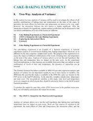
Figure 1 shows, however, that such asymptotics should be interpreted with some care. The
panels show the values of the sample median and MAD, together with the values of the Student
median, for simulated samples from the beta(.2,.2) and .5:.5 Gaussian mixture. The sample median/MAD
pair falls under the case originally addressed by Huber; their asymptotic distribution
is indeed Gaussian, with the diagonal variance matrix. Nevertheless, we clearly observe—in particular
in the left panel—that the dependence pattern is even stronger than that for the Student
median.
A bimodal situation like this is a trap for estimators with breakdown value 1/2. They behave
like Buridan’s Ass between two haystacks 1 : if purely deterministic, it would be starved to death
by its inability to choose among equally attractive alternatives. Stochastics saves the donkey—
but in repeated trials, both haystacks are visited about equally often. In technical terms, the
1 See, for instance, Blackburn, S.: The Oxford Dictionary of Philosophy, Oxford University Press, Oxford, 1996.

6
beta(.2,.2)
.5 N(−3,1) + .5 N(3,1)
σ
0.1 0.2 0.3 0.4 0.5
σ
1.5 2.0 2.5 3.0 3.5
0.0 0.2 0.4 0.6 0.8 1.0
µ
−3 −2 −1 0 1 2 3
µ
Figure 1. Median and MAD (•) and the Student median (+) from 100 samples
of size n = 100, drawn from the beta(.2,.2) distribution and .5:.5 random Gaussian
mixture.
result may be inconsistency, as demonstrated by Freedman and Diaconis (1982) for M-estimators
minimizing a non-convex function; see also Mizera (1994). Neither Student median with its
breakdown value 1/3, nor the sample median as an M-estimator minimizing a convex function
are formally covered by this theory; but even though they are both consistent, this phenomenon
results in inflated asymptotic variance.
Recall that the asymptotic variance of the sample median is inversely proportional to the
value of the density of the sampling distribution at the median. The density of beta(.2,.2) is
well beyond 0 at 0, hence the sample median performs well in this case. However, the value of
the density of the .5:.5 Gaussian mixture at 0 (three standard deviations from both means) is
very small. Note that in the last case, the Cauchy MLE, whose breakdown value is 1/2, does
not perform well either; only the Student median shows definite convergence (confirmed also by
larger sample sizes not shown here).
In the spirit of Theorem 4.1 of Mizera (2002), which says that bias sets are contained in deep
depth contours, a possible explanation could be that the simulated values of the Student median
tend to follow the shape of deeper contours—which in bimodal cases indeed have the crescentlike,
bent down form. Note also that it is hard to tell the quadratic fit from that by a circle arc
in the scale of a data cloud corresponding to n = 10000.
Table 2 shows that the behavior of the Student median scale is considerably simpler. The
MAD is always significantly worst, except for the sample size n = 10 from the .5:.5 Gaussian
mixture and the Cauchy distribution. The Student median scale is always either the best, or

7
n ˆσ N(0,1) Lap. Exp. Γ(.2) B(.2,1) B(.2,.2) 75:25 .5:.5 t(5) t(1)
sms 38319 69674 34120 1385 2465 15305 76253 821385 57478 520665
10 mad 48681 98262 44180 2966 4837 18754 146212 704780 77727 394011
cms 29924 61456 29090 2017 3301 13970 76894 590983 48717 285962
sms 13999 23106 11642 374 851 10137 28129 298772 19919 81604
30 mad 19889 33430 16450 518 1220 13284 47437 415810 27876 96892
cms 11732 20712 10923 376 937 8151 24735 326072 17228 74974
sms 4098 6639 3298 84 204 3385 9037 37388 5221 22071
100 mad 5841 9582 5013 143 318 5717 13869 149063 7220 25457
cms 3458 6074 3189 113 251 2392 7038 138963 4663 21417
sms 437 678 315 7 15 129 1017 1453 609 2073
1000 mad 568 963 503 12 25 557 1451 5932 806 2455
cms 357 635 318 9 20 76 762 10495 507 2016
Table 2. Estimated variance (×10 6 ) of the scale part of the Student median
(sms), the median absolute deviation from the median (mad), and the scale part
of location-scale Cauchy MLE (cms), for sample sizes n = 10, 30, 100, 1000.
only slightly worse than the Cauchy MLE scale; in any case, its estimated variance is smaller
than that of the MAD, except again for the two cases with n = 10 mentioned above.
Finally, we observe that the estimated variances of the Student median and the locationscale
Cauchy MLE differ—and the difference is in some cases, for instance for the .5:.5 normal
mixture, quite significant and grows with the sample size. This provides an evidence against
the contemplated asymptotic equivalence of the two estimators, albeit perhaps not conclusive—
random variability is a factor, and numerical artifacts are not impossible. Note also that the
breakdown value of the Cauchy MLE is 1/2, while that of the Student median 1/3.
2.5. Algorithmics. Not experts in the field, we really enjoyed Eppstein’s concise but exhaustive
explanation about time complexities, additional references to known algorithms, and illuminating
examples demonstrating the worst-case bounds. Concerning the practicalities, we do not
quarrel too much about whether to transform or not to transform in the actual implementation—
we believe that the final decision would likely depend also on programming and other conveniences.
In particular, it may well strongly favor simplicity. When worrying about rounding
errors, we had rather in mind Poincaré or Klein disks, where unbounded portions of the sample
are squeezed to finite segments; the parabolic lifting suggested by Eppstein seems to be much
less affected by this problem.
If the Student depth contours are computed for the continuous probability distributions
using our Theorem 9, then the approach without transformation is the only possible—since

it would be difficult to calculate the transformed distribution. The R library of functions
for computing sample and population Student depth contours, following closely the approach
of Theorems 8 and 9, was implemented by the second author and can be found at
http://www.member.uni-oldenburg.de/ch.mueller/packages.html.
In the time between the original paper and this rejoinder, the first author implemented the
simple O(n), apart from the initial O(n log n) sorting, algorithm for computing a sample Student
depth contour. All contours can be thus computed in O(n 2 ) time; let us remark that computing
all contours is seldom practical, since usually only a preselected number of contours is required.
The same algorithm is also used, combined with the binary search, for the computation of the
Student median depth contour; the resulting complexity is O(n log n).
The principal geometric operation in the Poincaré plane is computing the intersection of two
halfcircles. This is actually a linear problem; no transformation to any other model is necessary.
Moreover, the algorithm takes the advantage of a particular feature of Poincaré plane setting—
the order of µ coordinates on the real line. We agree with Eppstein that a conceptually simpler
solution might be to compute the Tukey depth for the parabolically lifted datapoints—in fact, we
would be happy to reuse the code generated by experts, but were not able to find readily available
software. So we chose the easiest path and implemented the algorithm for the Student depth contours
directly—since this problem is easier than the algorithm for two-dimensional depth contours
(even if its worst-case time complexity is the same). The C implementation of the algorithm is
a part of the R package LSD, available at http://www.stat.ualberta.ca/∼mizera/lsd.html.
The computation of the deepest contour for a sample of size n = 100000 takes on 1GHz PowerPC
G4 about 1.23 ± 0.15 and on 1GHz Pentium III about 2.26 ± 0.13 seconds. For such a sample
size, the result for a simulated sample gives practically the population depth contours of a given
distribution.
8
3. Potential extensions and ramifications
The discussants suggested a couple of interesting ideas concerning potential extensions and
ramifications of the Student depth and Student median.
3.1. Multivariate location and scale. Serfling is right: the extension to the multivariate
location-scale we had in mind would take the halfspace depth based on the criterial functions
derived from the multivariate Gaussian likelihood, resulting in
{
d(µ, Σ) =
inf
u∈R d ,v∈R d(d+1)/2
(u T ,v T )≠0
=‖
d∑
j≤k
i: u T Σ −1 (y i − µ) +
v jk
(− 1 2 tr(Σ−1 T jk ) + 1 ) }
2 (y i − µ) T Σ −1 T jk Σ −1 (y i − µ) ≥ 0 ,

where T jk is the d × d matrix whose all elements are 0 except for t jk = t kj = 1; see, for instance,
page 7 of Christensen (2001). This definition is really “straightforward, but somewhat technical”.
Less so is its geometrical interpretation—so far, we are able to describe only special cases, close
to that discussed by Eppstein.
If Σ is a diagonal matrix with diagonal elements σk 2 , then the just defined depth specializes to
d(µ, Σ) =
inf
u∈R d ,v∈R d
(u T ,v T )≠0
=‖ {i: y i ∈ H u,v } ,
with H u,v being the ellipsoid in R d given by
{
y ∈ R d : ( y − µ + Σ 1/2 V −1 u ) T
V Σ ( −1 y − µ + Σ 1/2 V −1 u ) }
≤ u T V −1 u + v T V −1 v ,
where V is the diagonal matrix with diagonal elements v 1 , . . . , v d . Consider the ellipsoid in R 2d
given by
{
(y T , z T ) T ∈ R 2d : ( y − µ + Σ 1/2 V −1 u ) T
V Σ ( −1 y − µ + Σ 1/2 V −1 u )
+ z T V Σ −1 z ≤ u T V −1 u + v T V −1 v } .
Then (µ T , 1 T d Σ1/2 ) T , where 1 d is the d-dimensional vector of ones, is an element of the boundary of
this ellipsoid. For d = 1, this characterizes the Student location-scale depth. However, for d > 1,
if some components of v, say l components, are equal to zero, then the geometrical structure
of H u,v is more complicated: the components of y that correspond to components of v that are
unequal to zero are lying in an ellipsoid of R d−l that has a size depending on the l components
of y that correspond to the vanishing components of v.
This problem does not appear in another special case, when Σ = σ 2 Σ 0 , where Σ 0 is a fixed
constant matrix and only σ 2 is a parameter. In this case, the tangent depth, with criterial
functions derived from the corresponding likelihood, is
d(µ, Σ) =
inf =‖ {i: y i ∈ H u,v } ,
u∈R d ,v∈R
u T Σ −1
0 u+v2 d=1
where H u,v is a halfspace for v = 0 and an ellipsoid or the complement of an ellipsoid in R d with
the boundary given for v ≠ 0 by
{ (
y ∈ R d : y − µ + σ )
v u T
Σ
−1
0
(y − µ + σ ) }
v u = σ2
.
v 2
In this case, d(µ, σ) is a hyperbolic Tukey depth. Moreover, the hyperbolic halfspaces H u,v have
the property that (µ 1 , . . . , µ d , σ √ d) T lies on the boundary of the ellipsoids in R d+1 given by
{
(
(y T , z) T ∈ R d+1 : y − µ + σ )
v u T
Σ
−1
0
(y − µ + σ ) }
v u + z 2 ≤ σ2
.
v 2
9

10
Conversely, if (µ 1 , . . . , µ d , σ √ d) T
lies on the boundary of an ellipsoid
then there exists (u T , v) T
{
(yT , z) T ∈ R d+1 : (y − λ) T Σ −1
0 (y − λ) + z 2 ≤ r 2} ,
∈ R d+1 with u T Σ −1
0 u + v 2 d = 1 such that the projected ellipsoid
{
y ∈ R d : (y − λ) T Σ −1
0 (y − λ) ≤ r 2}
coincides with H u,v . If Σ 0 is the unit diagonal matrix and v ≠ 0, then H u,v is the disk or the
complement of the disk with center y−µ+(uσ)/v and radius σ/v. The same holds if transformed
data ỹ i = Σ −1/2
0 y i are used. Since also the halfspaces can be interpreted as disks with infinite
radius, all sets H u,v can be viewed as disks or disk complements. Since (µ 1 , . . . , µ d , σ √ d) T and
not (µ 1 , . . . , µ d , σ) T lies on the boundary of the hemisphere in R d+1 with H u,v as its boundary,
the depth we obtained here is not exactly the hyperbolic Tukey depth proposed by Eppstein.
Nevertheless, Eppstein’s Theorem 1 can still be used to characterize it, after a small modification
of the set C: the depth of (µ 1 , . . . , µ d , σ) is equal to the minimum number of data points in a
closed disk or disk complement in R d bounded by a circle passing through two diametrically
opposed points of C = {ξ ∈ R d : |ξ − µ| = σ 2 d}. This depth is the hyperbolic Tukey depth with
respect to this C; all Eppstein’s characterizations for the hyperbolic Tukey depth hold also for
this depth, with σ 2 replaced by σ 2 d.
Despite the formal agreement at the end, as statisticians we have to remark that it may
be quite hard to envisage application for a multivariate problem where the variance-covariance
matrix is confined to the form σ 2 I—that is, the datapoints potentially come from a distribution
with possibly different locations, but the same scale in each coordinate.
3.2. Outlyingness and other extensions. Serfling also considered outlyingness-based proposals
of Zuo and Zhang, and contemplates possible connections and extensions. This is a very
interesting topic and deserves further investigation; the area is complex and cannot be handled
just in passing. Let us remark only that the theoretical properties are undoubtedly promising,
especially robustness (expressed through the breakdown value); efficiency may be an issue, but
given the progress in this direction achieved by other investigators, we believe that this is a
manageable task. However, the ultimate data-analytic success will, in our opinion, depend on
the availability of reliable and efficient algorithms—and this issue is still a pain, albeit not totally
without any treatment; see Remark 3.2 of Zuo et al. (2004).
Finally, Serfling also proposes several other alternatives for location and scale estimators,
whose interrelations, properties, and statistical utility may become interesting topics for further
research.
4. Fundamental questions: applications, interpretations
Last but not least, we must worry with McCullagh about how to put all of this to good
statistical use.

4.1. Estimation. Originally, we did not have too much hope in this particular line of
application—there is already a number of robust estimators, the location-scale context being
particularly abundant of them; despite all theory, very few of them are in practical use. But the
reaction of our discussants suggests that perhaps we might not be able to view the issue from
the right perspective.
Tables 1 and 2 suggest that as far as efficiency is concerned, the Student median is not worse,
and even sometimes better than the combined sample median/MAD pair. The advantage of the
latter is simplicity and 50% breakdown point. There are many better estimators indeed, but
few of them share the same conceptual clarity. Our examples and the simulations of He and
Portnoy show that the Student median can be viewed as giving results similar to the sample
median/MAD pair—but also as giving results significantly different in some cases. Thus, the
final attitude is somewhat in the eye of beholder.
In fact, we do not think the Student median completely lacks conceptual simplicity (there are
worse estimators in this respect). The issue of interpretability was raised by He and Portnoy;
albeit we do not have ready answers, let us offer at least a thought exercise, similar to that
used by Mizera and Volauf (2002). Concerning the population Student median, He and Portnoy
indicate that while the deepest regression estimates a meaningful quantity, the other maximum
depth estimators might be more problematic in this respect. However, before redirecting all this
negative outcome to the “genetically engineered” Student median, think of giving some share
also to the “traditional” (should we say “organic”?) Tukey median. Apart from the symmetry
issues clarified by Rousseeuw and Struyf (2004) and Zuo and Serfling (2000), what other kind
of understanding do we already have for it? An interpretation in “lay language”? We believe
that if one questions the meaning of the maximum depth estimators as generalized medians, the
Tukey median is a natural point to start.
One of more constructive paths leads through another lucid contribution of Hubert, Rousseeuw,
and Vanden Branden, who applied the symmetry considerations similar to those of Rousseeuw
and Struyf (2004) to the location-scale case and obtained a characterization of the invariance
of the distribution with respect to the transformation z → −1/z. Their result may offer one
possible explanation of the Student depth: for a given location-scale parameter, it measures its
invariance under this transformation—similarly as the Tukey depth may be viewed as measuring
the centrosymmetry of a given data point. Unfortunately, we are not (and were not) able to
see any immediate statistical interpretation of the examples, given by Hubert, Rousseeuw, and
Vanden Branden, of the distributions that are invariant with respect to this symmetry.
Finally, we want to stress that while some discussants (Serfling, He and Portnoy) tie the
Student depth with the Gaussian distribution, and others (Hubert, Rousseeuw, and Vanden
Branden) rather with the Cauchy distribution, it is the whole t family of distributions whose
scores generate the Student depth—not only its aforementioned extremes.
11

4.2. Testing. The simulation study conducted by He and Portnoy showed that the difference
between the depth of the Student median and the maximum depth at the median has a tendency
to attain larger values for asymmetric or bimodal distributions. This observation suggests a
possibility to use this difference for testing symmetry and/or unimodality; more generally, we
may consider a hypothesis in the general form (µ, σ) ∈ Θ 0 , where Θ 0 , for instance, may stand
for all (µ, σ) with µ = 0.
A convenient test of such a hypothesis can be based on the simplicial location-scale depth d S ,
which may be defined also via a generalized scheme involving any initial depth function d,
d s (ϑ; y 1 , . . . , y n ) = ( 1 ∑
n
1 {d(ϑ; yi1 ,...,y iq )>0}(y i1 , . . . , y iq );
q)
i 1

That said, let us just offer yet another example—provoked by the remark of He and Portnoy:
“whether this provides an improvement on QQ-plots is not clear”. Contrary to rather small
datasets we considered so far, our present example will involve two datasets, each containing
100000 datapoints. They were artificially generated—but we believe they may still illustrate
some phenomena arising in the exploratory data analysis of large datasets.
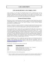
Figure 2 shows two quantile-quantile plots. Apparently, they exhibit no difference, except for
the size and number of the very few extreme outliers—a quite inessential phenomenon given the
large sample size. However, the corresponding plots of the Student depth contours—LSD-plots—
in Figure 3 reveal some difference.
Knowing that both datasets are simulated mixtures, we cannot decide whether this fact can
be convincingly inferred from the different shapes of inner and outer contour. But we believe
it is clear that both plots are different. Both datasets contain 80000 pseudorandom realizations
from the Cauchy distribution; the first one then contains 120000 standard Gaussian points, the
second one 60000 Gaussian with mean −2 and 60000 Gaussian with mean 2, both with standard
deviation 1.
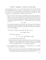
We emphasize the fact that Figure 3 shows LSD-plots in their default version, without any
additional tuning. After some experience, we tend now to think that less contours is more. Three,
however (as would correspond to a “location-scale boxplot”) are somewhat too few; six, at levels
i/6, give better information; and so does the “dozen” of them, at levels i/12, the alternative
that can be actually seen in Figure 3. (We always plot only nonempty contours, of course.) The
use of color is a working possibility—we are grateful to He and Portnoy for the particularly nice
“geographic” suggestion (not featured here for technical reasons).
We would like to dissuade any conception that LSD-plots might perhaps be intended to replace
some well-established tool. As practitioners know, no tool is universal; the best way is to use
13
Figure 2. The two quantile-quantile plots show only minor differences.

them in combination. So we offer LSD-plots as a possible addition to the array of graphical
exploratory techniques. There are not that many of them, at least not that many substantially
different—for some more esoteric ones, see Tukey (1990). Some of them are good in certain
situations, some in other. Our present example probably calls for a density estimate—but its
default application produces a very uninteresting picture, not worth of reproducing here. After
some effort—one has to compute the density estimate only from the datapoints lying within the
whiskers of a typical boxplot—we obtained the result showed in Figure 4. Conclusion? Albeit one
might think in this example that the density estimate eventually got it, we are pretty confident
there are examples where the outcome would go other way round. But in any case, the LSD-plots
definitely revealed somewhat more than the QQ-plots.
4.4. Geometry and Möbius invariance. After reviewing all immediate applications of the
location-scale depth, we get to the point when we dare to pronounce that perhaps the biggest
merit, if any, of them is that they potentially open a way of viewing the location-scale parameter
space, and consequently the data in a somewhat novel way. In this respect, probably the most
promising perspective is opened by the comment of McCullagh, who shows how the layering of
the parametric space induced by the Student depth could be used for more complex and appealing
tasks than just location and scale estimation. Even if his proposals do not use the location scale
depth directly (if we understand them well), but rather think in terms of the closely related
Cauchy MLE, they certainly deserve further thought. In this sense, McCullagh perhaps answers
14
6
6
6
6
5
5
5
5
4
4
4
4
σ
3
3
σ 3
3
2
2
2
2
1
1
1
1
0
−3 −2 −1 0 1 2 3
µ
0
0
−4 −2 0 2 4
µ
0
Figure 3. The corresponding LSD-plots show an apparent difference.

15
density(x = mx1, from = boxplot.stats(mx1)$s[1], to = boxplot.stats(mx1)$s[5])
density(x = mx2, from = boxplot.stats(mx2)$s[1], to = boxplot.stats(mx2)$s[5])
Density
0.05 0.10 0.15 0.20 0.25 0.30 0.35
Density
0.00 0.05 0.10 0.15
−3 −2 −1 0 1 2 3
N = 100000 Bandwidth = 0.103
−6 −4 −2 0 2 4 6
N = 100000 Bandwidth = 0.2299
Figure 4. The corresponding density estimates show even more, but only after
some effort: the estimates should be computed only for the datapoints lying within
the whiskers of their boxplot (not shown here).
our original question “what are the possible data-analytic uses of the new concept?” better than
we were able ourselves.
Having learned of Möbius invariance from McCullagh (1996), we find his query about its
statistical utility a bit surprising. But the question is a right one: as far as we can recall,
statistical textbooks deal with technical aspects of invariance and equivariance on the premise
that the desirability of those is somewhat self-explanatory. Indeed, invariance is seldom perceived
as a priori bad; it only starts to be a problem if it wreaks havoc with some other desirable
traits. (The first author remembers that a referee of one of his early papers studying location
estimators objected to translation equivariance on the grounds that Bayesian estimators with a
prior concentrated on a compact set do not possess it.)
In other words, invariance starts to be undesirable when it starts to be restrictive. Too stringent
requirements may result in trivial procedures; hence invariance with respect to rich classes of
transformations is generally known to fare well only in simple situations—in the location model,
for instance, the sample median is equivariant with respect to all monotone transformations. It
should be therefore mentioned that it is the line of methods derived from the halfspace depth
that opens new perspectives by showing extents of invariance which data analysis has not seen
yet; let us only mention a very strong property pointed out by Van Aelst et al. (2002), that
maximum regression depth fit is equivariant with respect to all monotone transformations of the
response.
While it seems that in the transition from location to location-scale we have to give up the
equivariance with respect to all monotone transformations, the Cauchy MLE and Student median
show that we may nevertheless add reciprocal values to translations and scalings. And McCullagh
further shows that the Möbius equivariance is achievable even in density estimation. In this
context, it is, in a sense, even more desirable than in the context of estimation; in the probabilistic

setting (note that our style of modeling dispensed with probabilities), Möbius equivariance of an
estimator is a natural requirement only if the parametric family of probabilities is closed under
Möbius transformation; the latter condition is, however, always true in density estimation.
If we, unlike Schervish (1995) or McCullagh (2002), try to think of equivariance just on very
primitive, data-analytic level by referring to measurement units, then the standard temperature
units, ◦ C, ◦ K, ◦ F, illustrate well a need of translation and rescaling. For the Möbius transformation,
a nice example is the way how automobile consumption is measured in North America
(miles per gallon) and in Europe (liters per 100 kilometers); note that this actually combines
the reciprocal with a rescaling. In physics, an example involving pure reciprocal transformation
could be electric resistance (measured in Ohms) versus conductivity (measured in Siemenses).
In fact, all physical units are expressed as products of integer (positive or negative) powers of
basic units—for instance, in the (metric) system of the physical units SI (Système International
d’unités).
At this point, it might thus look that Möbius should be enough. However, physicists also
work with quantities on logarithmic scales—for instance, the intensity of sound in acoustics
measured in decibels, or the magnitude of a star in astronomy. Here however, to accommodate
the logarithm into their system of dimensions, they rather divide by a reference quantity, to make
the problematic quantities dimensionless. So, who knows. In any case, the statistical meaning
of invariance and equivariance apparently deserves further study.
5. Conclusion
Given the space limitations, we were not able to address every raised issue. Certainly, the
difference between parameter and data depth, as pointed out by He and Portnoy, should be
given further thought. We are not able to answer their query about non- or semiparametric
fits; we are not there yet. But this discussion gives us a strong faith that we will get there one
day. We learned a lot, and also enjoyed it; we only hope that similarly did the discussants, and
eventually will the readers.
In addition to all discussants, we are grateful to the Associate Editor, and to the Editor
of JASA, Francisco J. Samaniego, for organizing this discussion. The research of Mizera was
supported by the Natural Sciences and Engineering Research Council of Canada; the research of
Müller, as well as her participation in JASA Theory and Methods Special Invited Paper session
at the Joint Statistical Meetings 2004 in Toronto, by Deutsche Forschungsgemeinschaft.
Additional References
Christensen, R. A. (2001), Advanced linear modeling, New York: Springer-Verlag.
Freedman, D. A. and Diaconis, P. (1982), “On inconsistent M-estimators,” Ann. Statist., 10,
454–461.
McCullagh, P. (2002), “What is a statistical model? (with discussion),” Ann. Statist., 30, 1225–
1310.
16

Mizera, I. (1994), “On consistent M-estimators: tuning constants, unimodality and breakdown,”
Kybernetika, 30, 289–300.
Schervish, M. J. (1995), Theory of Statistics, New York: Springer-Verlag.
Tukey, J. W. (1990), “Steps toward a universal univariate distribution analyzer,” in The Collected
Works of John W. Tukey VI, Belmont, CA: Wadsworth, pp. 585–590.
Zuo, Y., Cui, H., and He, X. (2004), “On the Stahel-Donoho estimator and depth-weighted
means of multivariate data,” Ann. Statist., 32, 167–188.
Zuo, Y. and Serfling, R. (2000), “On the performance of some robust nonparametric location
measures relative to a general notion of multivariate symmetry,” J. Statist. Plann. Inference,
84, 55–79.
previously cited (hence omitted in print):
Huber, P. J. (1981), Robust statistics, New York: John Wiley and Sons.
Liu, R. Y. (1988), “On a Notion of Simplicial Depth,” Proc. Nat. Acad. Sci., 85, 1732–1734.
— (1990), “On a Notion of Data Depth Based on Random Simplices,” Ann. Statist., 18, 405–414.
McCullagh, P. (1996), “Möbius Transformation and Cauchy Parameter Estimation,” Annals of
Statistics, 24, 787–808.
Mizera, I. (2002), “On depth and deep points: A calculus,” Ann. Statist., 30, 1681–1736.
Mizera, I. and Volauf, M. (2002), “Continuity of halfspace depth contours and maximum depth
estimators: diagnostics of depth-related methods,” J. Multivariate Anal., 83, 365–388.
Müller, C. H. (2003), “Depth estimators and tests based on the likelihood principle with application
to regression,” J. Multivariate Anal. in press.
Rousseeuw, P. J. and Struyf, A. (2004), “Characterizing angular symmetry and regression symmetry,”
J. Statist. Plann. Inference, 122, 161–173.
Van Aelst, S., Rousseeuw, P. J., Hubert, M., and Struyf, A. (2002), “The deepest regression
method,” J. Multiv. Analysis, 81, 138–166.
17