Chemical Process Control a First Course with Matlab

2 - 2
deviation variables—they denote how a quantity deviates from the original value at t = 0. 1
Since C o is a constant, we can rewrite Eq. (2-1) as
τ dC'
dt
+C' =C' in , with C'(0) = 0
(2-2)
Note that the equation now has a zero initial condition. For reference, the solution to Eq. (2-2) is 2
C'(t) = 1 τ
0
t
C' in
(z) e –(t–z)/τ dz
(2-3)
If C' in is zero, we have the trivial solution C' = 0. It is obvious from Eq. (2-2) immediately.
For a more interesting situation in which C' is nonzero, or for C to deviate from the initial C o ,
C' in must be nonzero, or in other words, C in is different from C o . In the terminology of differential
equations, the right hand side C' in is named the forcing function. In control, it is called the input.
Not only C' in is nonzero, it is under most circumstances a function of time as well, C' in = C' in (t).
In addition, the time dependence of the solution, meaning the exponential function, arises from
the left hand side of Eq. (2-2), the linear differential operator. In fact, we may recall that the left
hand side of (2-2) gives rise to the so-called characteristic equation (or characteristic polynomial).
Do not worry if you have forgotten the significance of the characteristic equation. We will
come back to this issue again and again. We are just using this example as a prologue. Typically
in a class on differential equations, we learn to transform a linear ordinary equation into an
algebraic equation in the Laplace-domain, solve for the transformed dependent variable, and
finally get back the time-domain solution with an inverse transformation.
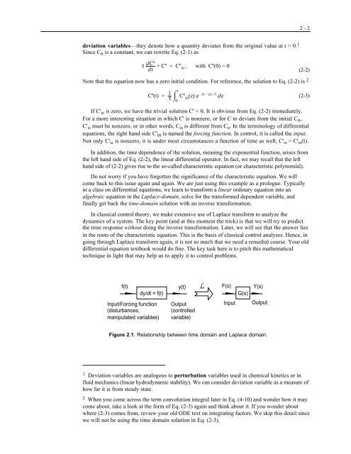
In classical control theory, we make extensive use of Laplace transform to analyze the
dynamics of a system. The key point (and at this moment the trick) is that we will try to predict
the time response without doing the inverse transformation. Later, we will see that the answer lies
in the roots of the characteristic equation. This is the basis of classical control analyses. Hence, in
going through Laplace transform again, it is not so much that we need a remedial course. Your old
differential equation textbook would do fine. The key task here is to pitch this mathematical
technique in light that may help us to apply it to control problems.
f(t) y(t) F(s) Y(s)
dy/dt = f(t)
G(s)
Input/Forcing function Output
Input Output
(disturbances,
(controlled
manipulated variables) variable)
L
Figure 2.1. Relationship between time domain and Laplace domain.
1 Deviation variables are analogous to perturbation variables used in chemical kinetics or in
fluid mechanics (linear hydrodynamic stability). We can consider deviation variable as a measure of
how far it is from steady state.
2 When you come across the term convolution integral later in Eq. (4-10) and wonder how it may
come about, take a look at the form of Eq. (2-3) again and think about it. If you wonder about
where (2-3) comes from, review your old ODE text on integrating factors. We skip this detail since
we will not be using the time domain solution in Eq. (2-3).