Chemical Process Control a First Course with Matlab
Chemical Process Control a First Course with Matlab
Chemical Process Control a First Course with Matlab
Create successful ePaper yourself
Turn your PDF publications into a flip-book with our unique Google optimized e-Paper software.
2 - 10<br />
2.5 Partial fraction expansion<br />
Since we rely on a look-up table to do reverse Laplace transform, we need the skill to reduce a<br />
complex function down to simpler parts that match our table. In theory, we should be able to<br />
"break up" a ratio of two polynomials in s into simpler partial fractions. If the polynomial in the<br />
denominator, p(s), is of an order higher than the numerator, q(s), we can derive 1<br />
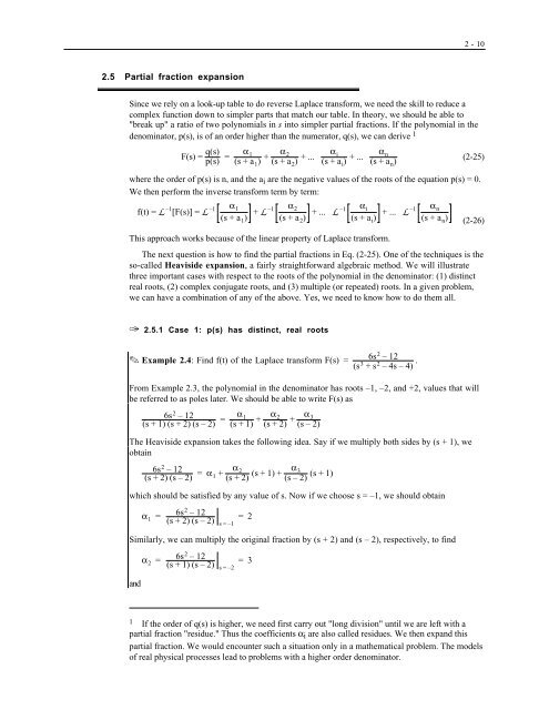
F(s) = q(s)<br />
p(s) = α 1<br />
(s + a 1 ) + α 2<br />
(s + a 2 ) + ... α i<br />
(s + a i ) + ... α n<br />
(s + a n )<br />
(2-25)<br />
where the order of p(s) is n, and the a i are the negative values of the roots of the equation p(s) = 0.<br />
We then perform the inverse transform term by term:<br />
f(t) = L –1 [F(s)] = L –1 α 1<br />
(s + a 1 )<br />
+ L –1 α 2<br />
(s + a 2 )<br />
+ ... L –1 α i<br />
(s + a i )<br />
+ ... L –1 α n<br />
(s + a n ) (2-26)<br />
This approach works because of the linear property of Laplace transform.<br />
The next question is how to find the partial fractions in Eq. (2-25). One of the techniques is the<br />
so-called Heaviside expansion, a fairly straightforward algebraic method. We will illustrate<br />
three important cases <strong>with</strong> respect to the roots of the polynomial in the denominator: (1) distinct<br />
real roots, (2) complex conjugate roots, and (3) multiple (or repeated) roots. In a given problem,<br />
we can have a combination of any of the above. Yes, we need to know how to do them all.<br />
✑ 2.5.1 Case 1: p(s) has distinct, real roots<br />
✎ Example 2.4: Find f(t) of the Laplace transform F(s) =<br />
6s 2 – 12<br />
(s 3 +s 2 – 4s – 4) .<br />
From Example 2.3, the polynomial in the denominator has roots –1, –2, and +2, values that will<br />
be referred to as poles later. We should be able to write F(s) as<br />
6s 2 – 12<br />
(s + 1) (s + 2) (s – 2) = α 1<br />
(s + 1) + α 2<br />
(s + 2) + α 3<br />
(s – 2)<br />
The Heaviside expansion takes the following idea. Say if we multiply both sides by (s + 1), we<br />
obtain<br />
6s 2 – 12<br />
(s + 2) (s – 2) = α 1 + α 2<br />
(s + 2) (s + 1) + α 3<br />
(s – 2)<br />
(s + 1)<br />
which should be satisfied by any value of s. Now if we choose s = –1, we should obtain<br />
α 1 =<br />
6s 2 – 12<br />
(s + 2) (s – 2) s=–1<br />
=2<br />
Similarly, we can multiply the original fraction by (s + 2) and (s – 2), respectively, to find<br />
α 2 =<br />
6s 2 – 12<br />
(s + 1) (s – 2) s=–2<br />
=3<br />
and<br />
1 If the order of q(s) is higher, we need first carry out "long division" until we are left <strong>with</strong> a<br />
partial fraction "residue." Thus the coefficients α i are also called residues. We then expand this<br />
partial fraction. We would encounter such a situation only in a mathematical problem. The models<br />
of real physical processes lead to problems <strong>with</strong> a higher order denominator.


