Chemical Process Control a First Course with Matlab

2 - 26
Let us try one simple example. Say if we keep the inlet temperature constant at our desired
steady state, the statement in deviation variable (without the apostrophe) is
T i (t) = 0 , and T i (s) = 0
Now we want to know what happens if the steam temperature increases by 10 °C. This change in
deviation variable is
T H = Mu(t) and T H (s) = M s
, where M = 10 °C
We can write
T(s) =
K p
τ p s+1
M
s (2-50)
After partial fraction expansion,
1
T(s) = MK p
s –
τ p
τ p
s+1
Inverse transform via table look-up gives our time-domain solution for the deviation in T: 1
T(t) = MK p 1 – e – t/τ p
(2-51)
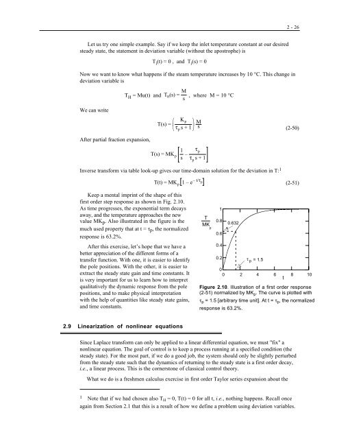
Keep a mental imprint of the shape of this
first order step response as shown in Fig. 2.10.
As time progresses, the exponential term decays
away, and the temperature approaches the new
value MK p . Also illustrated in the figure is the
much used property that at t = τp, the normalized
response is 63.2%.
After this exercise, let’s hope that we have a
better appreciation of the different forms of a
transfer function. With one, it is easier to identify
the pole positions. With the other, it is easier to
extract the steady state gain and time constants. It
is very important for us to learn how to interpret
qualitatively the dynamic response from the pole
positions, and to make physical interpretation
with the help of quantities like steady state gains,
and time constants.
1
p
T
MK
0.8
0.632
0.6
0.4
0.2
τ p = 1.5
0
0 2 4 6 8 10
t
Figure 2.10. Illustration of a first order response
(2-51) normalized by MK p . The curve is plotted with
τ p = 1.5 [arbitrary time unit]. At t = τ p , the normalized
response is 63.2%.
2.9 Linearization of nonlinear equations
Since Laplace transform can only be applied to a linear differential equation, we must "fix" a
nonlinear equation. The goal of control is to keep a process running at a specified condition (the
steady state). For the most part, if we do a good job, the system should only be slightly perturbed
from the steady state such that the dynamics of returning to the steady state is a first order decay,
i.e., a linear process. This is the cornerstone of classical control theory.
What we do is a freshmen calculus exercise in first order Taylor series expansion about the
1 Note that if we had chosen also T H = 0, T(t) = 0 for all t, i.e., nothing happens. Recall once
again from Section 2.1 that this is a result of how we define a problem using deviation variables.