Chemical Process Control a First Course with Matlab

3 - 2
are the two transfer functions for the two inputs X 1 (s) and X 2 (s).
Take note (again!) that the characteristic polynomials in the denominators of both transfer
functions are identical. The roots of the characteristic polynomial (the poles) are independent of
the inputs. It is obvious since they come from the same differential equation (same process or
system). The poles tell us what the time-domain solution, y(t), generally would "look" like. A
final reminder: no matter how high the order of n may be in Eq. (3-4), we can always use partial
fractions to break up the transfer functions into first and second order terms.
3.1 First order differential equation models
This section is a review of the properties of a first order differential equation model. Our Chapter 2
examples of mixed vessels, stirred-tank heater, and homework problems of isothermal stirred-tank
chemical reactors all fall into this category. Furthermore, the differential equation may represent
either a process or a control system. What we cover here applies to any problem or situation as
long as it can be described by a linear first order differential equation.
We usually try to identify features which are characteristic of a model. Using the examples in
Section 2.8 as a guide, a first order model using deviation variables with one input and with
constant coefficients a 1 , a o and b can be written in general notations as 1
The model, as in Eq. (2-2), is rearranged as
a 1
dy
dt +a o y = bx(t) with a 1 ≠ 0 and y(0) = 0 (3-5)
τ dy
dt
+y = Kx(t) (3-6)
where τ is the time constant, and K is the steady state gain.
In the event that we are modeling a process, we would use a subscript p (τ = τ p , K = K p ).
Similarly, the parameters would be the system time constant and system steady state gain when we
analyze a control system. To avoid confusion, we may use a different subscript for a system.
y
1.2
MK 1
0.8
0.6
0.4 increasing τ
0.2
0
0 2 4 6 8
t
10 12
2
K = 2
1.5
y
M
K = 1
1
0.5
K = 0.5
0
0 2 4 6 t 8 10
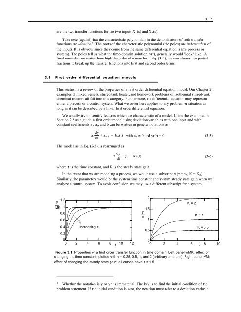
Figure 3.1. Properties of a first order transfer function in time domain. Left panel y/MK: effect of
changing the time constant; plotted with τ = 0.25, 0.5, 1, and 2 [arbitrary time unit]. Right panel y/M:
effect of changing the steady state gain; all curves have τ = 1.5.
1 Whether the notation is y or y‘ is immaterial. The key is to find the initial condition of the
problem statement. If the initial condition is zero, the notation must refer to a deviation variable.