describing function analysis of mechanical systems with nonlinear ...
describing function analysis of mechanical systems with nonlinear ...
describing function analysis of mechanical systems with nonlinear ...

Create successful ePaper yourself
Turn your PDF publications into a flip-book with our unique Google optimized e-Paper software.
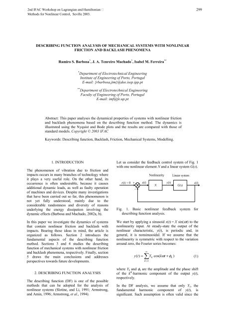
DESCRIBING FUNCTION ANALYSIS OF MECHANICAL SYSTEMS WITH NONLINEAR<br />
FRICTION AND BACKLASH PHENOMENA<br />
Ramiro S. Barbosa * , J. A. Tenreiro Machado * , Isabel M. Ferreira **<br />
* Department <strong>of</strong> Electrotechnical Engineering<br />
Institute <strong>of</strong> Engineering <strong>of</strong> Porto, Portugal<br />
E-mail: {rbarbosa,jtm}@dee.isep.ipp.pt<br />
** Department <strong>of</strong> Electrotechnical Engineering<br />
Faculty <strong>of</strong> Engineering <strong>of</strong> Porto, Portugal<br />
E-mail: imf@fe.up.pt<br />
Abstract: This paper analyses the dynamical properties <strong>of</strong> <strong>systems</strong> <strong>with</strong> <strong>nonlinear</strong> friction<br />
and backlash phenomena based on the <strong>describing</strong> <strong>function</strong> method. The dynamics is<br />
illustrated using the Nyquist and Bode plots and the results are compared <strong>with</strong> those <strong>of</strong><br />
standard models. Copyright © 2003 IFAC<br />
Keywords: Describing <strong>function</strong>, Backlash, Friction, Mechanical Systems, Modelling.<br />
1. INTRODUCTION<br />
The phenomenon <strong>of</strong> vibration due to friction and<br />
impacts occurs in many branches <strong>of</strong> technology where<br />
it plays a very useful role. On the other hand, its<br />
occurrence is <strong>of</strong>ten undesirable, because it causes<br />
additional dynamic loads, as well as faulty operation<br />
<strong>of</strong> machines and devices. Despite many investigations<br />
that have been carried out so far, this phenomenon is<br />
not yet fully understood, mainly due to the<br />
considerable randomness and diversity <strong>of</strong> reasons<br />
underlying the energy dissipation involving the<br />
dynamic effects (Barbosa and Machado, 2002a, b).<br />
In this paper we investigate the dynamics <strong>of</strong> <strong>systems</strong><br />
that contain <strong>nonlinear</strong> friction and backlash <strong>with</strong><br />
impacts. Bearing these ideas in mind, the article is<br />
organized as follows. Section 2 introduces the<br />
fundamental aspects <strong>of</strong> the <strong>describing</strong> <strong>function</strong><br />
method. Sections 3 and 4 studies the <strong>describing</strong><br />
<strong>function</strong> <strong>of</strong> <strong>mechanical</strong> <strong>systems</strong> <strong>with</strong> <strong>nonlinear</strong> friction<br />
and backlash phenomena, respectively. Finally, section<br />
5 draws the main conclusions and addresses<br />
perspectives towards future developments.<br />
2. DESCRIBING FUNCTION ANALYSIS<br />
The <strong>describing</strong> <strong>function</strong> (DF) is one <strong>of</strong> the possible<br />
methods that can be adopted for the <strong>analysis</strong> <strong>of</strong><br />
<strong>nonlinear</strong> <strong>systems</strong> (Slotine, and Li, 1991; Armstrong,<br />
and Amin, 1996; Armstrong, et al., 1994).<br />
Let us consider the feedback control system <strong>of</strong> Fig. 1<br />
<strong>with</strong> one <strong>nonlinear</strong> element N and a linear system G(s).<br />
r(t) = 0<br />
+<br />
−<br />
x(t)<br />
Nonlinearity<br />
N<br />
y(t)<br />
Linear system<br />
G(s)<br />
Fig. 1. Basic <strong>nonlinear</strong> feedback system for<br />
<strong>describing</strong> <strong>function</strong> <strong>analysis</strong>.<br />
We start by applying a sinusoid x(t) = X sin(ωt) to the<br />
<strong>nonlinear</strong>ity input. At steady-state the output <strong>of</strong> the<br />
<strong>nonlinear</strong> characteristic, y(t), is periodic and, in<br />
general, it is nonsinusoidal. If we assume that the<br />
<strong>nonlinear</strong>ity is symmetric <strong>with</strong> respect to the variation<br />
around zero, the Fourier series becomes:<br />
y(<br />
t)<br />
=<br />
∑ ∞<br />
k =1<br />
Y<br />
k<br />
z(t)<br />
cos( kω t + φ )<br />
(1)<br />
where Y k and φ k are the amplitude and the phase shift<br />
<strong>of</strong> the k th -harmonic component <strong>of</strong> the output y(t),<br />
respectively.<br />
In the DF <strong>analysis</strong>, we assume that only Y 1 , the<br />
fundamental harmonic component <strong>of</strong> y(t), is<br />
significant. Such assumption is <strong>of</strong>ten valid since the<br />
k
higher-harmonics in y(t), Y k for k = 2, 3, …, are usually<br />
<strong>of</strong> smaller amplitude than the amplitude <strong>of</strong> the<br />
fundamental component Y 1 . Moreover, most <strong>systems</strong><br />
are “low-pass filters” <strong>with</strong> the result that the higherharmonics<br />
are further attenuated.<br />
Input force F<br />
M<br />
x , x&<br />
Thus the DF <strong>of</strong> a <strong>nonlinear</strong> element, N(X,ω), is defined<br />
as the complex ratio <strong>of</strong> the fundamental harmonic<br />
component <strong>of</strong> output y(t) <strong>with</strong> the input x(t):<br />
a)<br />
Friction force F f<br />
1<br />
N X = (2)<br />
(<br />
, ω)<br />
Y1<br />
e<br />
X<br />
where X is the amplitude <strong>of</strong> the input sinusoid x(t) and<br />
Y 1 and φ 1 are the amplitude and the phase shift <strong>of</strong> the<br />
fundamental harmonic component <strong>of</strong> the output y(t),<br />
respectively.<br />
In general, N(X,ω) is a <strong>function</strong> <strong>of</strong> both the amplitude<br />
X and the frequency ω <strong>of</strong> the input sinusoid. For<br />
<strong>nonlinear</strong> <strong>systems</strong> that do not involve energy storage,<br />
the DF is merely amplitude-dependent, that is<br />
N = N(X). If it is not the case, we may have to adopt a<br />
numerical approach because, usually, it is impossible<br />
to find a closed-form solution.<br />
For the <strong>nonlinear</strong> control system <strong>of</strong> Fig. 1, we have a<br />
limit cycle if the sinusoid at the <strong>nonlinear</strong>ity input<br />
regenerates itself in the loop, that is:<br />
jφ<br />
1<br />
G(<br />
jω)<br />
= −<br />
(3)<br />
N(<br />
X , ω)<br />
Note that (3) can be viewed as the characteristic<br />
equation <strong>of</strong> the <strong>nonlinear</strong> feedback system <strong>of</strong> Fig. 1. If<br />
(3) can be satisfied for some value <strong>of</strong> X and ω, a limit<br />
cycle is predicted for the <strong>nonlinear</strong> system. Moreover,<br />
since (3) applies only if the <strong>nonlinear</strong> system is in a<br />
steady-state limit cycle, the DF <strong>analysis</strong> predicts only<br />
the presence or the absence <strong>of</strong> a limit cycle and cannot<br />
be applied to <strong>analysis</strong> for other types <strong>of</strong> time<br />
responses.<br />
3. SYSTEMS WITH NONLINEAR FRICTION<br />
This section analyses the DF <strong>of</strong> a dynamical system<br />
<strong>with</strong> <strong>nonlinear</strong> friction (Haessig, and Friedland, 1991;<br />
Armstrong, et al., 1994; Azenha, and Machado, 1998).<br />
The system under consideration is a simple mass<br />
system <strong>with</strong> Coulomb plus Viscous plus Static friction<br />
(CVS model) as represented in Fig. 2.<br />
The equation <strong>of</strong> motion in this system is as follows:<br />
M& x<br />
( t)<br />
+ Ff ( t)<br />
= f ( t)<br />
(4)<br />
where M is the system mass, F f (t) is the friction force<br />
and f(t) the applied input force.<br />
Friction force F f<br />
F s<br />
F c<br />
b)<br />
- F c<br />
Velocity x&<br />
- F s<br />
Fig. 2. a) Elemental mass system subjected to<br />
<strong>nonlinear</strong> friction and b) Coulomb plus viscous<br />
plus static friction (CVS) model.<br />
The discontinuity at zero velocity <strong>of</strong> the CVS model<br />
may lead to numerical problems in the simulations. To<br />
overcome the zero crossing detection and to get a<br />
reasonable numerical robustness we adopt the Karnopp<br />
model (Karnopp, 1985). The advantage <strong>of</strong> this model<br />
is that can produce sufficiently accurate results while<br />
reducing the algorithm complexity and simulation<br />
time. This model is described as:<br />
F<br />
f<br />
( x&<br />
F)<br />
( x&<br />
)<br />
⎧ Fc<br />
sgn + Bx&<br />
, x&<br />
> Dv<br />
, = ⎨<br />
(5)<br />
⎩min( F , Fs<br />
) sgn( F)<br />
, x&<br />
≤ Dv<br />
where D v specifies a small neighbourhood <strong>of</strong> the zero<br />
velocity (Karnopp, 1985).The parameters F c , F s and B<br />
are respectively the Coulomb, Static and Viscous<br />
friction level.<br />
For the simple system <strong>of</strong> Fig. 2a we can calculate,<br />
numerically, the Nyquist plot <strong>of</strong> −1/N(F,ω)<br />
considering as input an sinusoidal force<br />
f(t) = F cos(ωt) applied to mass M and as output the<br />
position x(t). Fig. 3 shows the <strong>function</strong> −1/N(F,ω) for<br />
several values <strong>of</strong> F.<br />
The values <strong>of</strong> the parameters used in the simulations<br />
are: M = 1 Kg, B = 0.5 Ns/m, F c = 5 N and F s = 7 N. In<br />
the subsequent results the linear system case is also<br />
plotted for comparison purposes.
0<br />
ω=30<br />
-2000 ω=40<br />
ω=50<br />
-4000<br />
ω=60<br />
linear<br />
F=50<br />
F=40<br />
F=30<br />
F=20<br />
10<br />
5<br />
Im (-1/N)<br />
-6000<br />
-8000<br />
-10000<br />
ω=70<br />
ω=80<br />
ω=90<br />
ω=100<br />
F=10<br />
-12000<br />
0 2000 4000 6000 8000 10000 12000 14000<br />
Re (-1/N)<br />
x(t)<br />
0<br />
-5<br />
-10<br />
65 70 75 80 85 90 95<br />
time (s)<br />
Fig. 3. Nyquist plot <strong>of</strong> −1/N(F,ω) for the system<br />
subjected to <strong>nonlinear</strong> friction and for an input<br />
force F = {10, 20, 30, 40, 50} N.<br />
Fig. 4 illustrates the variation <strong>of</strong> the Nyquist plots <strong>of</strong><br />
−1/N(F,ω) for the cases <strong>of</strong> the linear system and<br />
<strong>nonlinear</strong> friction. The log-log plots <strong>of</strong> Re{−1/N} and<br />
Im{−1/N} vs. the exciting frequency ω, for different<br />
values <strong>of</strong> the input force F = {10, 20, 30, 40, 50} N,<br />
reveal that we get results closer to the linear case the<br />
higher the excitation force F, particularly for the real<br />
component.<br />
|Re (-1/N)|<br />
10 4<br />
10 2<br />
10 0<br />
F=10 F=50<br />
Fig. 5. Time response <strong>of</strong> the output position x(t) <strong>of</strong><br />
the system <strong>with</strong> <strong>nonlinear</strong> friction <strong>with</strong> ω = 0.5<br />
rad/s, for F = 10 N (solid line) and F = 50 N<br />
(dashed line, scaled down by a factor <strong>of</strong> 10).<br />
Log(|F(x(t))|)<br />
10<br />
5<br />
0<br />
-5<br />
-10<br />
10 2<br />
10 1<br />
10 0<br />
ω (rad/s)<br />
10 -1<br />
10 -2<br />
0<br />
F=10 N<br />
1 2<br />
a)<br />
F=50 N<br />
3 4 5<br />
6 7<br />
8 9 10<br />
harmonic index k<br />
10 6 ω (rad/s)<br />
|Im (-1/N)|<br />
10 -2<br />
linear<br />
10 -4<br />
10 -2 10 -1 10 0 10 1 10 2<br />
10 4<br />
10 2<br />
F=10<br />
F=50<br />
10 0<br />
linear<br />
10 -2<br />
10 -4<br />
10 -2 10 -1 10 0 10 1 10 2<br />
10 6 ω (rad/s)<br />
Log(|F(x(t))|)<br />
10<br />
5<br />
0<br />
-5<br />
10 2<br />
10 1<br />
10 0<br />
ω (rad/s)<br />
10 -1<br />
10 -2<br />
0 1 2 3 4 5 6 7 8 9 10<br />
harmonic index k<br />
b)<br />
Fig. 6. Fourier transform <strong>of</strong> the output position x(t),<br />
F{x(t)}, over 20 cycles, vs. (ω, k), the exciting<br />
frequency ω and the harmonic frequency index k<br />
for: a) An input force F = 10 N and b) An input<br />
force F = 50 N.<br />
Fig. 4. Log-log plots <strong>of</strong> Re{−1/N} and Im{−1/N} vs.<br />
the exciting frequency ω, for F = {10, 20, 30, 40,<br />
50} N.<br />
Fig. 5 compares the time response for an input force<br />
<strong>of</strong> F = 10 N and F = 50 N. We conclude that for low<br />
forces the <strong>nonlinear</strong> effects <strong>of</strong> the static and Coulomb<br />
frictions are more significant, which is in accordance<br />
<strong>with</strong> the signal harmonic content F{x(t)} depicted in<br />
Fig.6.
4. SYSTEMS WITH BACKLASH AND IMPACTS<br />
In this section, we use the DF method to analyse the<br />
phenomena <strong>of</strong> clearance <strong>with</strong>out and <strong>with</strong> the effect <strong>of</strong><br />
the impacts, usually called static backlash and<br />
dynamic backlash, respectively (Barbosa, and<br />
Machado, 2002b; Nordin, and Gutman, 2002;<br />
Stepanenko, and Sankar, 1986; Dubowsky, et al.,<br />
1987; Choi, and Noah, 1989; Tao, and Kokotovic,<br />
1995).<br />
The standard approach to the backlash study is based<br />
on the adoption <strong>of</strong> a geometric model that neglects the<br />
dynamic phenomena involved during the impact<br />
process. Due to this reason <strong>of</strong>ten real results differ<br />
significantly from those predicted by that model.<br />
The static backlash model leads to a DF <strong>of</strong> a linear<br />
system <strong>of</strong> a single mass M 1 +M 2 followed by the<br />
geometric backlash having as input and as output the<br />
position variables x(t) and y(t), respectively, as<br />
depicted in Fig. 7a.<br />
The <strong>describing</strong> <strong>function</strong> for X > h/2 is given by<br />
(Phillips and Harbour, 2000):<br />
k ⎡ ⎛ X / h ⎞⎤<br />
2kh(<br />
X − h / 2)<br />
N(<br />
X ) = 1 N s<br />
j<br />
2<br />
⎢ − ⎜ ⎟ −<br />
1 X / h<br />
⎥<br />
2<br />
⎣ ⎝ − ⎠⎦<br />
πX<br />
(6)<br />
2 ⎡ −1<br />
1 1 ⎛ −1<br />
1 ⎞⎤<br />
N s ( z)<br />
= ⎢sin<br />
+ cos⎜sin<br />
⎟<br />
π<br />
⎥<br />
⎣ z z ⎝ z ⎠⎦<br />
(7)<br />
For the dynamic backlash, the proposed <strong>mechanical</strong><br />
model consists on two masses (M 1 and M 2 ) subjected<br />
not only to backlash but also to impact phenomena as<br />
shown in Fig. 7b.<br />
Linear system<br />
f(t) 1<br />
x(t) slope k y(t)<br />
-h/2<br />
f(t)<br />
( M + M ) s<br />
2<br />
Side<br />
A<br />
1<br />
G(s)<br />
x 1 , x&<br />
1<br />
2<br />
x 2, x&<br />
M 2<br />
M 1<br />
2<br />
a)<br />
b)<br />
Backlash<br />
h<br />
y<br />
N(X)<br />
h/2 x<br />
Side<br />
B<br />
Fig. 7. a) Classic backlash model and b) System <strong>with</strong><br />
two masses subjected to dynamic backlash.<br />
A collision between the masses M 1 and M 2 occurs<br />
when x 1 = x 2 or x 2 = h + x 1 . In this case, we can<br />
compute the velocities <strong>of</strong> masses M 1 and M 2 after the<br />
impact ( x′ & 1 and x′ & 2 ) by relating them to the previous<br />
values ( x&<br />
1 and x&<br />
2 ) through Newton’s law:<br />
( x ′ − x&<br />
′ ) = −ε<br />
( x&<br />
− x&<br />
),<br />
0 ≤ ε 1<br />
& (8)<br />
1 2 1 2 ≤<br />
where ε is the coefficient <strong>of</strong> restitution. In the case <strong>of</strong><br />
a fully plastic (inelastic) collision ε = 0, while in the<br />
ideal elastic case ε = 1.<br />
By application <strong>of</strong> the principle <strong>of</strong> conservation <strong>of</strong><br />
momentum M 1x& 1′ + M 2 x&<br />
2′<br />
= M1x&<br />
1 + M 2 x&<br />
2 and <strong>of</strong><br />
expression (8), we can find the sought velocities <strong>of</strong><br />
both masses after an impact:<br />
x&<br />
( M − ε M ) + x&<br />
( 1 + ε )<br />
1 1 2 2<br />
2<br />
x& 1′<br />
=<br />
(9)<br />
M1<br />
+ M 2<br />
x&<br />
M<br />
( 1 + ε ) M + x&<br />
( M − εM<br />
)<br />
1 1 2 2 1<br />
x& 2′<br />
=<br />
(10)<br />
M1<br />
+ M 2<br />
For the system <strong>of</strong> Fig. 7b we calculate numerically<br />
the Nyquist diagram <strong>of</strong> −1/N(F,ω) for an input force<br />
f(t) = F cos(ωt) applied to mass M 2 and considering<br />
the output position x 1 (t) <strong>of</strong> mass M 1 .<br />
The values <strong>of</strong> the parameters adopted in the<br />
subsequent simulations are: M 1 = M 2 = 1 Kg and<br />
h = 10 −1 m. Figs. 8 and 9 show the Nyquist plots for<br />
F = 50 N and ε = {0.1, …, 0.9} and for F = {10, 20,<br />
30, 40, 50} N and ε = {0.2, 0.8}, respectively.<br />
The Nyquist charts <strong>of</strong> Figs. 8−9 reveal the occurrence<br />
<strong>of</strong> a jumping phenomenon, which is a characteristic<br />
<strong>of</strong> <strong>nonlinear</strong> <strong>systems</strong>. This phenomenon is more<br />
visible around ε ≈ 0.5, while for the limiting cases<br />
(ε → 0 and ε → 1) the singularity disappears.<br />
Moreover, Fig. 8 shows also that for a fixed value <strong>of</strong><br />
ε the charts are proportional to the input amplitude F.<br />
The validity <strong>of</strong> the model is restricted to an input<br />
force f(t) <strong>with</strong> frequency higher than a lower-limit<br />
ω C ≈ [(2F / M 2 h) 2 (1−ε) 5 ] 1/4 and lower than an upperlimit<br />
ω L = 2(F / M 2 h) 1/2 , corresponding to an<br />
amplitude <strong>of</strong> x 1 (t) <strong>with</strong>in the clearance h/2. In the<br />
middle-range, ω C < ω < ω L , occurs a jumping<br />
phenomena at frequency ω J ~ (F / M 2 h) 1/2 .<br />
Fig. 10 illustrates the variation <strong>of</strong> the Nyquist plots <strong>of</strong><br />
−1/N(F,ω) for the cases <strong>of</strong> the static and dynamic<br />
backlash and shows the log-log plots <strong>of</strong> Re{−1/N}<br />
and Im{−1/N} vs. ω for an input force F = 50 N and<br />
ε = {0.1, 0.3, 0.5, 0.7, 0.9}.<br />
Comparing the results for the static and the dynamic<br />
backlash models we conclude that:<br />
• The charts <strong>of</strong> Re{−1/N} are similar for low<br />
frequencies (where they reveal a slope <strong>of</strong> +40
dB/dec) but differ significantly for high<br />
frequencies;<br />
• The charts <strong>of</strong> Im{−1/N} are different in all<br />
range <strong>of</strong> frequencies. Moreover, for low<br />
frequencies, the dynamic backlash has a<br />
fractional slope inferior to +80 dB/dec <strong>of</strong> the<br />
static model.<br />
Re(-1/N)<br />
10 3<br />
10 2<br />
10 1<br />
Static<br />
ε =0.7, 0.9<br />
ε =0.5<br />
ε =0.3<br />
ε =0.1<br />
3000<br />
Dynamic<br />
2500<br />
ε =0.1<br />
10 4 ω (rad/s)<br />
10 0<br />
Im (-1/N)<br />
2000<br />
1500<br />
1000<br />
ε =0.2<br />
ω=40<br />
ω=35<br />
ω=30<br />
ε =0.3<br />
ε =0.4<br />
ε =0.5<br />
ε =0.6<br />
ω=25<br />
ε =0.7<br />
500<br />
ε =0.8<br />
ω=20<br />
ε =0.9<br />
ω=15<br />
0<br />
ε→1<br />
-500 0 500 1000 1500 2000<br />
Re(-1/N)<br />
Im (-1/N)<br />
10 -1<br />
10 3<br />
10 2<br />
10 1<br />
10 0<br />
10 0 10 1 10 2<br />
Static<br />
ε =0.1<br />
ε =0.3<br />
ε =0.5<br />
ε =0.7<br />
ε =0.9<br />
Dynamic<br />
10 4 ω (rad/s)<br />
Fig. 8. Nyquist plot <strong>of</strong> −1/N(F,ω) for the dynamic<br />
backlash, F = 50 N and ε = {0.1, …, 0.9}.<br />
10 -1<br />
10 -2<br />
Im(-1/N)<br />
2500<br />
2000<br />
1500<br />
1000<br />
500<br />
F=10<br />
ε =0.2<br />
F=20<br />
F=30<br />
F=40<br />
F=50<br />
ω=25<br />
ω=40<br />
ω=20<br />
ω=15<br />
0<br />
0 200 400 600 800 1000<br />
Re(-1/N)<br />
ω=35<br />
ω=30<br />
10 -3<br />
10 0 10 1 10 2<br />
Fig. 10. Log-log plots <strong>of</strong> Re{−1/N} and Im{−1/N} vs.<br />
the exciting frequency ω, for F = 50 N and<br />
ε = {0.1, 0.3, 0.5, 0.7, 0.9}.<br />
Fig. 11 shows the time response <strong>of</strong> the output<br />
velocity x& ( ) <strong>of</strong> a system <strong>with</strong> dynamic backlash for<br />
1 t<br />
ω = {20, 40} rad/s and ε = {0.2, 0.8} revealing that<br />
we can have either chaotic or periodic responses<br />
depending on the values <strong>of</strong> ω and ε.<br />
2<br />
400<br />
1.5<br />
350<br />
ε =0.8<br />
F=50<br />
1<br />
Im(-1/N)<br />
300<br />
250<br />
200<br />
150<br />
F=20<br />
F=30<br />
F=40<br />
ω=30<br />
ω=35<br />
ω=40<br />
dx 1<br />
/dt<br />
0.5<br />
0<br />
−0.5<br />
−1<br />
100<br />
50<br />
F=10<br />
ω=20<br />
ω=25<br />
ω=15<br />
0<br />
0 200 400 600 800 1000 1200 1400 1600 1800<br />
Re(-1/N)<br />
Fig. 9. Nyquist plots <strong>of</strong> −1/N(F,ω) for a system <strong>with</strong><br />
dynamic backlash, F = {10, 20, 30, 40, 50} N and<br />
ε = {0.2, 0.8}.<br />
−1.5<br />
1.65 1.7 1.75 1.8 1.85 1.9 1.95 2 2.05 2.1<br />
time(s)<br />
Fig. 11. Time response <strong>of</strong> the output velocity x&<br />
1(<br />
t)<br />
<strong>of</strong><br />
the system <strong>with</strong> dynamic backlash, F = 50 N for<br />
ω = 20 rad/s, ε = 0.8 (solid line) and ω = 40 rad/s,<br />
ε = 0.2 (dotted line).<br />
Fig. 12 presents the Fourier transform <strong>of</strong> the output<br />
displacement <strong>of</strong> mass M 1 , F{x 1 (t)}, namely the<br />
amplitude <strong>of</strong> the harmonic content <strong>of</strong> x 1 (t) for an input<br />
force f(t) = 50 cos(ωt), ω C < ω < ω L , and ε = {0.2, 0.8}.<br />
The charts reveal that the fundamental harmonic <strong>of</strong> the
output has a much higher magnitude than the other<br />
higher-harmonic components. This fact enables the<br />
application <strong>of</strong> the <strong>describing</strong> <strong>function</strong> in the prediction<br />
<strong>of</strong> limit cycles for this system. Nevertheless, for high<br />
values <strong>of</strong> ε, there is a significant high-order harmonic<br />
content, and by consequence, a lower precision <strong>of</strong> the<br />
limit cycle prediction.<br />
Log(|F(x 1<br />
(t))|)<br />
Log(|F(x 1<br />
(t))|)<br />
0<br />
-5<br />
-10<br />
40<br />
30<br />
20<br />
ω (rad/s)<br />
5<br />
0<br />
-5<br />
-10<br />
10<br />
50<br />
40<br />
ω (rad/s) 30<br />
20<br />
10<br />
0<br />
0<br />
0<br />
1<br />
ε=0.2<br />
2<br />
a)<br />
3<br />
ε=0.8<br />
4<br />
10<br />
6<br />
7<br />
8<br />
9<br />
5<br />
harmonic index k<br />
0 1 2 3 4 5 6 7 8 9 10<br />
harmonic index k<br />
b)<br />
Fig. 12. Fourier transform <strong>of</strong> the output displacement<br />
x 1 (t), F{x 1 (t)}, over 20 cycles, vs. the exciting<br />
frequency ω and the harmonic index k for: a) An<br />
restitution coefficient ε = 0.2 and b) An<br />
restitution coefficient ε = 0.8.<br />
5. CONCLUSIONS<br />
This paper addressed several aspects <strong>of</strong> the phenomena<br />
involved in <strong>systems</strong> <strong>with</strong> <strong>nonlinear</strong> friction and<br />
backlash. The dynamics <strong>of</strong> elemental <strong>mechanical</strong><br />
system was analysed through the <strong>describing</strong> <strong>function</strong><br />
method and compared <strong>with</strong> standard models. The<br />
results encourage further studies <strong>of</strong> <strong>nonlinear</strong> <strong>systems</strong><br />
in a similar perspective and the <strong>analysis</strong> <strong>of</strong> limit cycle<br />
prediction. The conclusion may lead to the<br />
development <strong>of</strong> compensation schemes capable <strong>of</strong><br />
improving control system performance.<br />
REFERENCES<br />
Armstrong-Hélouvry, B. and B. Amin (1996). PID<br />
Control in the Presence <strong>of</strong> Static Friction: A<br />
Comparison <strong>of</strong> Algebraic and Describing<br />
Function Analysis. Automatica, 32, 679−692.<br />
Armstrong-Hélouvry, B., P. Dupont and C. Canudas<br />
de Wit (1994). A Survey <strong>of</strong> Models, Analysis<br />
Tools and Compensation Methods for the<br />
Control <strong>of</strong> Machines <strong>with</strong> Friction. Automatica,<br />
30, 1083−1138.<br />
Azenha, A. and J. A. T. Machado (1998). On the<br />
Describing Function Method and the Prediction<br />
<strong>of</strong> Limit Cycles in Nonlinear Dynamical<br />
Systems. SAMS Journal <strong>of</strong> Systems Analysis,<br />
Modelling and Simulation, 33, 307−320.<br />
Barbosa, R. S. and J. T. Machado (2002a). Fractional<br />
Describing Function Analysis <strong>of</strong> Systems <strong>with</strong><br />
Backlash and Impact Phenomena. In: Proc. <strong>of</strong><br />
the 6 th Int. Conf. on Intelligent Engineering<br />
Systems 2002, pp. 521−526. Opatija, Croatia.<br />
Barbosa, R. S. and J. T. Machado (2002b).<br />
Describing Function Analysis <strong>of</strong> Systems <strong>with</strong><br />
Impacts and Backlash. Nonlinear Dynamics, 29,<br />
235−250.<br />
Choi, Y. S. and S. T. Noah (1989). Periodic Response<br />
<strong>of</strong> a Link Coupling <strong>with</strong> Clearance. ASME<br />
Journal <strong>of</strong> Dynamic Systems, Measurement and<br />
Control, 111, 253−259.<br />
Dubowsky, S., J. F. Deck and H. Costello (1987).<br />
The Dynamic Modelling <strong>of</strong> Flexible Spatial<br />
Machine Systems <strong>with</strong> Clearance Connections.<br />
ASME Journal <strong>of</strong> Mechanisms, Transmissions<br />
and Automation in Design, 109, 87−94.<br />
Haessig, D. A. Jr. and B. Friedland (1991). On the<br />
Modeling and Simulation <strong>of</strong> Friction. ASME<br />
Journal <strong>of</strong> Dynamic Systems, Measurement and<br />
Control, 113, 354−362.<br />
Karnopp, D. (1985). Computer Simulation <strong>of</strong> Stick-<br />
Slip Friction in Mechanical Dynamic Systems.<br />
ASME Journal <strong>of</strong> Dynamic Systems,<br />
Measurement and Control, 107, 100−103 .<br />
Nordin, M. and P. Gutman (2002). Controlling<br />
Mechanical Systems <strong>with</strong> Backlash−A Survey.<br />
Automatica, 38, 1633−1649.<br />
Phillips, C. L. and R. D. Harbor (2000). Feedback<br />
Control Systems. Prentice-Hall, New Jersey.<br />
Slotine, J. E. and W. Li (1991). Applied Nonlinear<br />
Control. Prentice-Hall, New Jersey.<br />
Stepanenko, Y. and T. S. Sankar (1986). Vibro-<br />
Impact Analysis <strong>of</strong> Control Systems <strong>with</strong><br />
Mechanical Clearance and its Aplication to<br />
Robotic Actuators. ASME Journal <strong>of</strong> Dynamic<br />
Systems, Measurement and Control, 108, 9−16.<br />
Tao, G. and P. V. Kokotovic. Adaptive Control <strong>of</strong><br />
Systems <strong>with</strong> Unknown Output Backlash (1995).<br />
IEEE Transactions on Automatic Control, 40,<br />
326−330.