describing function analysis of mechanical systems with nonlinear ...

higher-harmonics in y(t), Y k for k = 2, 3, …, are usually
of smaller amplitude than the amplitude of the
fundamental component Y 1 . Moreover, most systems
are “low-pass filters” with the result that the higherharmonics
are further attenuated.
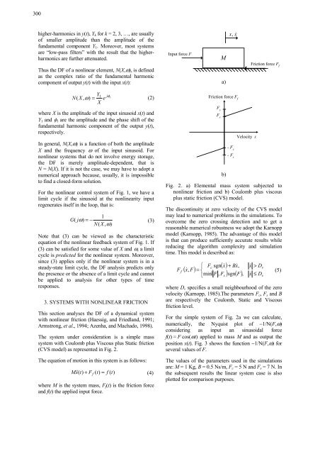
Input force F
M
x , x&
Thus the DF of a nonlinear element, N(X,ω), is defined
as the complex ratio of the fundamental harmonic
component of output y(t) with the input x(t):
a)
Friction force F f
1
N X = (2)
(
, ω)
Y1
e
X
where X is the amplitude of the input sinusoid x(t) and
Y 1 and φ 1 are the amplitude and the phase shift of the
fundamental harmonic component of the output y(t),
respectively.
In general, N(X,ω) is a function of both the amplitude
X and the frequency ω of the input sinusoid. For
nonlinear systems that do not involve energy storage,
the DF is merely amplitude-dependent, that is
N = N(X). If it is not the case, we may have to adopt a
numerical approach because, usually, it is impossible
to find a closed-form solution.
For the nonlinear control system of Fig. 1, we have a
limit cycle if the sinusoid at the nonlinearity input
regenerates itself in the loop, that is:
jφ
1
G(
jω)
= −
(3)
N(
X , ω)
Note that (3) can be viewed as the characteristic
equation of the nonlinear feedback system of Fig. 1. If
(3) can be satisfied for some value of X and ω, a limit
cycle is predicted for the nonlinear system. Moreover,
since (3) applies only if the nonlinear system is in a
steady-state limit cycle, the DF analysis predicts only
the presence or the absence of a limit cycle and cannot
be applied to analysis for other types of time
responses.
3. SYSTEMS WITH NONLINEAR FRICTION
This section analyses the DF of a dynamical system
with nonlinear friction (Haessig, and Friedland, 1991;
Armstrong, et al., 1994; Azenha, and Machado, 1998).
The system under consideration is a simple mass
system with Coulomb plus Viscous plus Static friction
(CVS model) as represented in Fig. 2.
The equation of motion in this system is as follows:
M& x
( t)
+ Ff ( t)
= f ( t)
(4)
where M is the system mass, F f (t) is the friction force
and f(t) the applied input force.
Friction force F f
F s
F c
b)
- F c
Velocity x&
- F s
Fig. 2. a) Elemental mass system subjected to
nonlinear friction and b) Coulomb plus viscous
plus static friction (CVS) model.
The discontinuity at zero velocity of the CVS model
may lead to numerical problems in the simulations. To
overcome the zero crossing detection and to get a
reasonable numerical robustness we adopt the Karnopp
model (Karnopp, 1985). The advantage of this model
is that can produce sufficiently accurate results while
reducing the algorithm complexity and simulation
time. This model is described as:
F
f
( x&
F)
( x&
)
⎧ Fc
sgn + Bx&
, x&
> Dv
, = ⎨
(5)
⎩min( F , Fs
) sgn( F)
, x&
≤ Dv
where D v specifies a small neighbourhood of the zero
velocity (Karnopp, 1985).The parameters F c , F s and B
are respectively the Coulomb, Static and Viscous
friction level.
For the simple system of Fig. 2a we can calculate,
numerically, the Nyquist plot of −1/N(F,ω)
considering as input an sinusoidal force
f(t) = F cos(ωt) applied to mass M and as output the
position x(t). Fig. 3 shows the function −1/N(F,ω) for
several values of F.
The values of the parameters used in the simulations
are: M = 1 Kg, B = 0.5 Ns/m, F c = 5 N and F s = 7 N. In
the subsequent results the linear system case is also
plotted for comparison purposes.