describing function analysis of mechanical systems with nonlinear ...

0
ω=30
-2000 ω=40
ω=50
-4000
ω=60
linear
F=50
F=40
F=30
F=20
10
5
Im (-1/N)
-6000
-8000
-10000
ω=70
ω=80
ω=90
ω=100
F=10
-12000
0 2000 4000 6000 8000 10000 12000 14000
Re (-1/N)
x(t)
0
-5
-10
65 70 75 80 85 90 95
time (s)
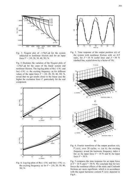
Fig. 3. Nyquist plot of −1/N(F,ω) for the system
subjected to nonlinear friction and for an input
force F = {10, 20, 30, 40, 50} N.
Fig. 4 illustrates the variation of the Nyquist plots of
−1/N(F,ω) for the cases of the linear system and
nonlinear friction. The log-log plots of Re{−1/N} and
Im{−1/N} vs. the exciting frequency ω, for different
values of the input force F = {10, 20, 30, 40, 50} N,
reveal that we get results closer to the linear case the
higher the excitation force F, particularly for the real
component.
|Re (-1/N)|
10 4
10 2
10 0
F=10 F=50
Fig. 5. Time response of the output position x(t) of
the system with nonlinear friction with ω = 0.5
rad/s, for F = 10 N (solid line) and F = 50 N
(dashed line, scaled down by a factor of 10).
Log(|F(x(t))|)
10
5
0
-5
-10
10 2
10 1
10 0
ω (rad/s)
10 -1
10 -2
0
F=10 N
1 2
a)
F=50 N
3 4 5
6 7
8 9 10
harmonic index k
10 6 ω (rad/s)
|Im (-1/N)|
10 -2
linear
10 -4
10 -2 10 -1 10 0 10 1 10 2
10 4
10 2
F=10
F=50
10 0
linear
10 -2
10 -4
10 -2 10 -1 10 0 10 1 10 2
10 6 ω (rad/s)
Log(|F(x(t))|)
10
5
0
-5
10 2
10 1
10 0
ω (rad/s)
10 -1
10 -2
0 1 2 3 4 5 6 7 8 9 10
harmonic index k
b)
Fig. 6. Fourier transform of the output position x(t),
F{x(t)}, over 20 cycles, vs. (ω, k), the exciting
frequency ω and the harmonic frequency index k
for: a) An input force F = 10 N and b) An input
force F = 50 N.
Fig. 4. Log-log plots of Re{−1/N} and Im{−1/N} vs.
the exciting frequency ω, for F = {10, 20, 30, 40,
50} N.
Fig. 5 compares the time response for an input force
of F = 10 N and F = 50 N. We conclude that for low
forces the nonlinear effects of the static and Coulomb
frictions are more significant, which is in accordance
with the signal harmonic content F{x(t)} depicted in
Fig.6.