B Trees

Purpose:
− understand the notion of B trees
− to build, in C, a B tree
1 2-3 Trees
1.1 General Presentation
Laboratory Module 8
B Trees
When working with large sets of data, it is often not possible or desirable to maintain the entire
structure in primary storage (RAM). Instead, a relatively small portion of the data structure is maintained in
primary storage, and additional data is read from secondary storage as needed. Unfortunately, a magnetic
disk, the most common form of secondary storage, is significantly slower than random access memory
(RAM). In fact, the system often spends more time retrieving data than actually processing data.
B-trees are balanced trees that are optimized for situations when part or all of the tree must be
maintained in secondary storage such as a magnetic disk. Since disk accesses are expensive (time
consuming) operations, a b-tree tries to minimize the number of disk accesses. For example, a b-tree with a
height of 2 and a branching factor of 1001 can store over one billion keys but requires at most two disk
accesses to search for any node.
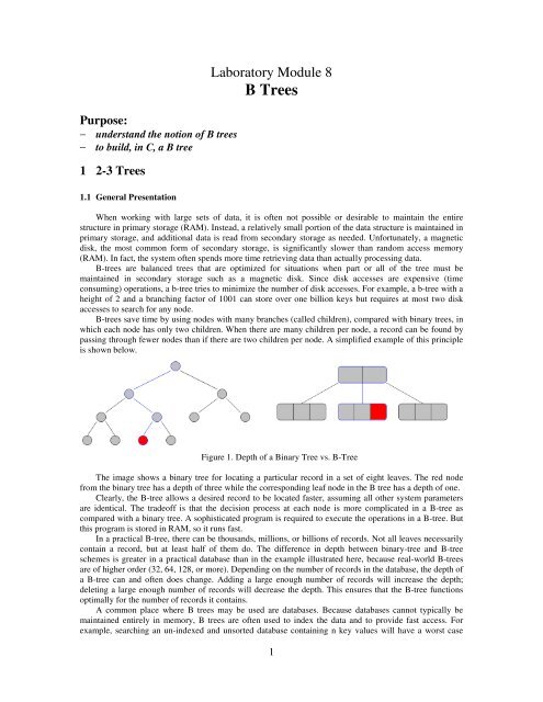
B-trees save time by using nodes with many branches (called children), compared with binary trees, in
which each node has only two children. When there are many children per node, a record can be found by
passing through fewer nodes than if there are two children per node. A simplified example of this principle
is shown below.
Figure 1. Depth of a Binary Tree vs. B-Tree
The image shows a binary tree for locating a particular record in a set of eight leaves. The red node
from the binary tree has a depth of three while the corresponding leaf node in the B tree has a depth of one.
Clearly, the B-tree allows a desired record to be located faster, assuming all other system parameters
are identical. The tradeoff is that the decision process at each node is more complicated in a B-tree as
compared with a binary tree. A sophisticated program is required to execute the operations in a B-tree. But
this program is stored in RAM, so it runs fast.
In a practical B-tree, there can be thousands, millions, or billions of records. Not all leaves necessarily
contain a record, but at least half of them do. The difference in depth between binary-tree and B-tree
schemes is greater in a practical database than in the example illustrated here, because real-world B-trees
are of higher order (32, 64, 128, or more). Depending on the number of records in the database, the depth of
a B-tree can and often does change. Adding a large enough number of records will increase the depth;
deleting a large enough number of records will decrease the depth. This ensures that the B-tree functions
optimally for the number of records it contains.
A common place where B trees may be used are databases. Because databases cannot typically be
maintained entirely in memory, B trees are often used to index the data and to provide fast access. For
example, searching an un-indexed and unsorted database containing n key values will have a worst case
1

unning time of O(n); if the same data is indexed with a b-tree, the same search operation will run in O(log
n). To perform a search for a single key on a set of one million keys (1,000,000), a linear search will
require at most 1,000,000 comparisons. If the same data is indexed with a b-tree of minimum degree 10,
114 comparisons will be required in the worst case. Clearly, indexing large amounts of data can
significantly improve search performance. Although other balanced tree structures can be used, a b-tree
also optimizes costly disk accesses that are of concern when dealing with large data sets.
The B-tree is also used in filesystems to allow quick random access to an arbitrary block in a particular
file.
1.1.1 Definition
A B-tree of order m (the maximum number of children for each node) is a tree which satisfies the
following properties:
1. Every node has at most m children.
2. Every node (except root and leaves) has at least m⁄2 children.
3. The root has at least two children if it is not a leaf node.
4. All leaves appear in the same level, and carry information.
5. A non-leaf node with k children contains k–1 keys.
Example:
Figure 2. Sample B Tree of order 2
Some balanced trees store values only at the leaf nodes, and so have different kinds of nodes for leaf
nodes and internal nodes. B-trees keep values in every node in the tree, and may use the same structure for
all nodes. However, since leaf nodes never have children, a specialized structure for leaf nodes in B-trees
will improve performance.
Unlike a binary-tree, each node of a b-tree may have a variable number of keys and children. The keys
are stored in non-decreasing order. Each key has an associated child that is the root of a subtree containing
all nodes with keys less than or equal to the key but greater than the preceding key. A node also has an
additional rightmost child that is the root for a subtree containing all keys greater than any keys in the node.
• Each internal node's elements act as separation values which divide its subtrees. For example, if an
internal node has three child nodes (or subtrees) then it must have two separation values or elements a 1 and
a 2 . All values in the leftmost subtree will be less than a 1 , all values in the middle subtree will be between
a 1 and a 2 , and all values in the rightmost subtree will be greater than a 2 .
• Each internal node of a B-tree will contain a number of keys. Usually, the number of keys is
chosen to vary between d and 2d. In practice, the keys take up the most space in a node. The factor of 2
will guarantee that nodes can be split or combined. If an internal node has 2d keys, then adding a key to
that node can be accomplished by splitting the 2d key node into two d key nodes and adding the key to the
parent node
• Internal nodes in a B-tree — nodes which are not leaf nodes — are usually represented as an
ordered set of elements and child pointers. Every internal node contains a maximum of U children and —
other than the root — a minimum of L children. For all internal nodes other than the root, the number
of elements is one less than the number of child pointers; the number of elements is between L-1 and U-
1. The number U must be either 2L or 2L-1; thus each internal node is at least half full. This
relationship between U and L implies that two half-full nodes can be joined to make a legal node, and one
full node can be split into two legal nodes (if there is room to push one element up into the parent). These
2

properties make it possible to delete and insert new values into a B-tree and adjust the tree to preserve the
B-tree properties.
• Leaf nodes have the same restriction on the number of elements, but have no children, and no
child pointers.
• The number of branches (or child nodes) from a node will be one more than the number of
keys stored in the node.
• A B-tree is kept balanced by requiring that all leaf nodes are at the same depth. This depth will
increase slowly as elements are added to the tree, but an increase in the overall depth is infrequent, and
results in all leaf nodes being one more node further away from the root.
• A B-tree of depth n+1 can hold about U times as many items as a B-tree of depth n, but the cost of
search, insert, and delete operations grows with the depth of the tree. As with any balanced tree, the cost
grows much more slowly than the number of elements.
• Considering ‘m’ the maximum number of offspring we will have the following declaration:
typedef struct NodeB {
int nr;
int key[m+1];
struct node *pchildren[m+1];
}pnode;
Figure 3. The structure of a node from a B tree
For n greater than or equal to one, the height of an n-key b-tree T of height h with a minimum degree t
greater than or equal to 2,
The worst case height is O(log n). Since the "branchiness" of a b-tree can be large compared to many
other balanced tree structures, the base of the logarithm tends to be large; therefore, the number of nodes
visited during a search tends to be smaller than required by other tree structures. Although this does not
affect the asymptotic worst case height, b-trees tend to have smaller heights than other trees with the same
asymptotic height.
1.2 Operations on B Trees
On a B-tree we can perform the following basic operations: Search, Insert, Delete.
Since all nodes are assumed to be stored in secondary storage (disk) rather than primary storage
(memory), all references to a given node be preceded by a read operation denoted by Disk-Read. Similarly,
once a node is modified and it is no longer needed, it must be written out to secondary storage with a write
operation denoted by Disk-Write.
1.2.1 Searching a Key
The search operation on a b-tree is analogous to a search on a binary tree. Instead of choosing between
a left and a right child as in a binary tree, a b-tree search must make an n-way choice. The correct child is
chosen by performing a linear search of the values in the node. After finding the value greater than or equal
to the desired value, the child pointer to the immediate left of that value is followed. If all values are less
than the desired value, the rightmost child pointer is followed. Of course, the search can be terminated as
soon as the desired node is found. Since the running time of the search operation depends upon the height
of the tree, B-Tree-Search is O(log n).
3

Figure 4. Searching key 38 in a B-Tree
The B-Tree search algorithm
The B-tree search algorithm takes as input a pointer to the root node “x” of a subtree and the key
“k ” which represents the key needed to be found. If the value is found in the B-tree, the algorithm
returns the ordered pair (y, i), consisting of a node “y” and an index “i” such that KEYi[y]=k.
Otherwise the value NIL is returned
PROCEDURE B-TREE-SEARCH (x , k)
begin
i=1
while ( i key i [x] )
do ( i

Example: Insertion in B-trees
Initial B-tree :
B-tree after the insertion ok key 2:
B-tree after the insertion of keys 3 and 4:
B-tree after the insertion of key 5:
B-tree after the insertion of keys 6 and 7:
B-tree after the insertion of key 8:
B-tree after the insertion of keys 9 and 10:
B-tree after the insertion of key11:
B-tree after the insertion of keys 12 and 13:
5

B-tree after the insertion of key 14:
B-tree after the insertion of keys 15 and 16:
B-tree after the insertion of key 17:
PROCEDURE B-TREE-INSERT(T, k)
begin
r = root[T]
if ( n[r] == 2t – 1){
s

do c j+1 [x] = c j [x]
c i+1 [x]= z
for ( j = n[x] downto i)
do key j+1 [x] = key j [x]
key i [x] = key t [y]
n[x] = n[x] + 1
Disk-Write(y)
Disk-Write(z)
Disk-Write(x)
end;
PROCEDURE B-TREE-INSERT-NONFULL ( x, k)
begin
i = n[x]
if ( leaf[x] )
then{
while( i >= 1 and k < key i [x] )
do{
key i +1[x] = key i [x])
i = i – 1
}//end do
key i+1 [x] = k
n[x] = 1 and k < key i [x] )
do i = i - 1
i = i + 1
Disk-Read(c i [x])
if ( n[c i [x]] == 2t – 1)
then {
B-Tree-Split-Child( x, i, c i [x])
if ( k > key i [x] )
then i

The insertion of the key 16 leads to the the node with keys 10, 12, 14 and 17 which exceeds the
maximum limit of the the tree, so we need to split the page into two smaller pages.
Figure 6b. The nodes involved in the split
1.2.3 Deleting a Key
Figure 6c. The B-tree after the insertion of key 16
Deletion of a key from a b-tree is possible; however, special care must be taken to ensure that the
properties of a b-tree are maintained.
There are two popular strategies for deletion from a B-Tree.
- locate and delete the item, then restructure the tree to regain its invariants
- do a single pass down the tree, but before entering (visiting) a node, restructure the tree so that
once the key to be deleted is encountered, it can be deleted without triggering the need for any
further restructuring
There are two special cases to consider when deleting an element:
1. the element in an internal node may be a separator for its child nodes
2. deleting an element may put its node under the minimum number of elements and children.
1.2.3.1 Deleting from a leaf node
The necessary steps for deleting from a leaf node are:
Step 1. Search for the value to delete.
Step 2. If the value is in a leaf node, it can simply be deleted from the node,
Step 3. If underflow happens, check siblings to either transfer a key or fuse the siblings together.
Step 4. If deletion happened from right child retrieve the max value of left child if there is no
underflow in left child. In vice-versa situation retrieve the min element from right.
Example: Deletion of key 3 from a B-Tree of order 2. Every page, except the root page, can contain
between 2 and 4 keys.If we want to delete key 3 we must first perform a search:
Figure 7a. Search operation for finding the key needed to be deleted
8

1.2.3.2 Deletion from an internal node
Figre 7b. The result of the deletion
Each element in an internal node acts as a separation value for two subtrees, and when such an element
is deleted, two cases arise. In the first case, both of the two child nodes to the left and right of the deleted
element have the minimum number of elements, namely L-1. They can then be joined into a single node
with 2L-2 elements, a number which does not exceed U-1 and so is a legal node. Unless it is known that
this particular B-tree does not contain duplicate data, we must then also (recursively) delete the element in
question from the new node.
In the second case, one of the two child nodes contains more than the minimum number of elements.
Then a new separator for those subtrees must be found. Note that the largest element in the left subtree is
still less than the separator. Likewise, the smallest element in the right subtree is the smallest element
which is still greater than the separator. Both of those elements are in leaf nodes, and either can be the new
separator for the two subtrees.
• If the value is in an internal node, choose a new separator (either the largest element in the left
subtree or the smallest element in the right subtree), remove it from the leaf node it is in, and
replace the element to be deleted with the new separator.
• This has deleted an element from a leaf node, and so is now equivalent to the previous case.
Example:
If we want to delete key 19 from the above-mentioned tree we perform the following operations:
Figure 8a. Searching the largest element in the left subtree (predecessor)
Figure 8b. The B-tree after the deletion of key 19
9

If deleting an element from a leaf node has brought it under the minimum size, some elements must be
redistributed to bring all nodes up to the minimum. In some cases the rearrangement will move the
deficiency to the parent, and the redistribution must be applied iteratively up the tree, perhaps even to the
root. Since the minimum element count doesn't apply to the root, making the root be the only deficient node
is not a problem. The algorithm to rebalance the tree is as follows:
• If the right sibling has more than the minimum number of elements
o Add the separator to the end of the deficient node.
o Replace the separator in the parent with the first element of the right sibling.
o Append the first child of the right sibling as the last child of the deficient node
• Otherwise, if the left sibling has more than the minimum number of elements.
o Add the separator to the start of the deficient node.
o Replace the separator in the parent with the last element of the left sibling.
o Insert the last child of the left sibling as the first child of the deficient node
• If both immediate siblings have only the minimum number of elements
o Create a new node with all the elements from the deficient node, all the elements from
one of its siblings, and the separator in the parent between the two combined sibling
nodes.
o Remove the separator from the parent, and replace the two children it separated with the
o
combined node.
If that brings the number of elements in the parent under the minimum, repeat these steps
with that deficient node, unless it is the root, since the root may be deficient.
The only other case to account for is when the root has no elements and one child. In this case it is
sufficient to replace it with its only child.
Example:
B-Tree-Delete-Key(x, k)
if ( not leaf[x] ) {
y = Preceding-Child(x)
z = Successor-Child(x)
if ( n[y] > t – 1 ) {
k ’ = Find-Predecessor-Key (k, x)
Move-Key(k’, y, x)
Move-Key(k, x, z)
B-Tree-Delete-Key(k, z)
}else
if ( n[z] > t – 1) {
k ’ = Find-Successor-Key(k, x)
Figure 9. Rebalancing after deletion
10

}else {
Move-Key(k ’ , z, x)
Move-Key(k, x, y)
B-Tree-Delete-Key(k, y)
Move-Key(k, x, y)
Merge-Nodes(y, z)
B-Tree-Delete-Key(k, y)
}
}else { // leaf node
y = Preceding-Child(x)
z = Successor-Child(x)
w= root(x)
v= RootKey(x)
if ( n[x] > t – 1){
Remove-Key( k, x )
}else {
if ( n[y] > t – 1 ) {
k = Find-Predecessor-Key (w, v)
Move-Key( k’, y, w)
k’ =Find-Successor-Key(w, v)
Move-Key(k’,w, x)
B-Tree-Delete-Key(k, x)
} else {
if ( n[w] > t – 1){
k’ = Find-Successor-Key(w, v)
Move-Key(k’, z,w)
k’ =Find-Predecessor-Key(w, v)
Move-Key(k’,w, x)
B-Tree-Delete-Key(k, x)
}else{
s = Find-Sibling(w)
w’ = root(w)
if ( n[w’] = t – 1) {
Merge-Nodes(w’,w)
Merge-Nodes(w, s)
B-Tree-Delete-Key(k, x)
} else {
Move-Key(v,w, x)
B-Tree-Delete-Key(k, x)
}
}
}
}
}
In the deleting procedure we have the following functions:
Preceding-Child(x) - Returns the left child of key x.
Move-Key(k, n1, n2) - Moves key k from node n1 to node n2.
Merge-Nodes(n1, n2) - Merges the keys of nodes n1 and n2 into a new node.
Find-Predecessor-Key(n, k) - Returns the key preceding key k in the child of node n.
Remove-Key(k, n) - Deletes key k from node n. n must be a leaf node.
11

2. Assignments
1) Consider the following B-tree of order 5:
Perform the following operations on the above-mentioned B-tree:
• Search for key 21;
• Insert key 28;
• Insert key 33;
• Delete key 6;
• Delete key 25
• Delete key 4;
2) Consider the following B-tree of order 5:
Perform the following operations on the above-mentioned B-tree:
• Search for key 24;
• Insert key 20;
• Insert key 6;
• Insert key 47;
• Delete key 13;
• Delete key 37;
• Delete key 19;
For each insertion operation there must be presented the following:
- Initial position of the key into the B tree
- Analysis regarding the number of keys
- The necessary movements of the keys (all necesary splits)
- The final shape of the tree
For each deletion operation there must be presented the following:
- The search of the tree for the key that needs to be deleted
- The analysis regarding the type (internal or root) of the node
- The necessary movements of the keys
- The final shape of the tree
12