Precision Stabilization Simulation of a Ball Joint Gimbaled Mirror ...

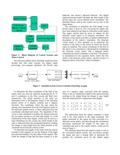
Figure 2. Block Diagram of Control Systems and
Motor Control
The ball-joint gimbal mirror Simulink model has been
divided into four main systems, the digital signal
processing, servo-capstan operation, the Kevlar rope
behavior, and mirror’s physical behavior. The digital
signal processing model calculates the final length of the
Kevlar ropes for a given desired mirror orientation. The
Simulink blocks used in this system can be seen in the
figure below.
The calculation to determine the final length of the
Kevlar ropes is done by first converting the angles that
have been entered as the input to a direction cosine matrix.
The angles entered must be given in radians for the
direction cosine matrix to be properly calculated. The
direction cosine matrix provides a complete mathematical
description of the mirror’s orientation. The direction
cosine matrix is then operated on to determine the
location of the holes in the mirror to which the Kevlar
ropes are attached. The current coordinates of the hole in
the mirror’s new orientation is determined by multiplying
the direction cosine matrix with a diagonal matrix
containing the initial coordinates of the hole. This process
is summarized by the equations below where the first
matrix is the direction cosine matrix, and the second is a
diagonal matrix of the holes’ initial coordinates.
Figure 3. Simulink System Used to Calculate Final Rope Length
To determine the final coordinates of the hole in the
mirror each row must be summed, producing the X, Y,
and Z coordinates in the first, second and third rows
respectively. The initial positions of the holes are
determined from a Pro/Engineer model of the ball-joint
gimbal mirror at 0 degrees azimuth and 0 degrees
elevation. The coordinates where the rope meets the
capstan, also determined from the Pro/Engineer model of
the ball-joint gimbal mirror, is then subtracted from the
coordinates calculated previously. The magnitude of this
vector is then calculated to produce the distance between
the two points, giving us our final rope length. To avoid
initialization of the rope lengths, which may be seen as a
large disturbance by the system, the initial length of the
rope is subtracted from the commanded position, yielding
the change in rope length from the initial position as the
command received by the control system.
To determine the lengths of the ropes from the optical
encoders in the capstans we use the measure of the angle
provided and multiply it by the radius of the capstan. This
yields the length of rope that has been wound, or in the
case of a negative angle, unwound, from the capstan.
There is also no initialization added to the optical encoder,
resulting in the output being the change in rope length
from the initial position’s appropriate rope lengths.
⎡uˆ
⎢
⎢
uˆ
⎢⎣
uˆ
x
y
z
vˆ
x
vˆ
y
vˆ
z
wˆ
x ⎤ ⎡X
i
wˆ
⎥
×
⎢
y
⎥ ⎢
0
wˆ
⎥⎦
⎢
z ⎣ 0
0
Y
i
0
0 ⎤ ⎡X
⎢
0
⎥
⎥
= ⎢ Y
Z ⎥⎦
⎢
i ⎣ Z
xx
yx
zx
X
Y
Z
xy
yy
zy
X
X
Z
xz
yz
zz
⎤
⎥
⎥
⎥
⎦
(1)
The information from the optical controller is dealt
with in the same fashion as the input command. The
angles measured by the sensor are first converted to a
direction cosine matrix, and then through the calculations
previously mentioned the lengths of the ropes are
calculated and sent to the control system, which can be
seen in Figure 4.
The resulting signal from the control system is sent to
the servomotor-capstan system. The servomotor accepts
the signal and uses a lookup table to determine the
position the command given by the digital signal