Precision Stabilization Simulation of a Ball Joint Gimbaled Mirror ...

Precision Stabilization Simulation of a Ball
Joint Gimbaled Mirror Using Advanced MATLAB ® Techniques
Orlando J. Hernandez
Electrical & Computer Engineering
The College of New Jersey
hernande@tcnj.edu
John A. Alamia
Electrical & Computer Engineering
Drexel University
alamia3@tcnj.edu
Abstract
With the increasing use of smart weapons and sensors,
there is a need to consider potential areas of improvement
that could positively affect large numbers of systems with
common concepts and approaches. One area that lends
itself to this desire is the improvement of high precision
high bandwidth antenna and mirror steering systems that
can be utilized across a broad range of sensor systems.
Pointing and tracking motions of typical antenna/mirror
systems have been accomplished using gimbaled control
systems in one or more axes. While these systems
generally exhibit high dynamic range, and excellent
accuracy and precision, they suffer from the common
problems of weight and power requirements, and
mechanical envelope constraints. This paper presents
techniques and results for the simulation of stabilization
characteristics of a joint gimbaled mirror using advanced
MATLAB tools and packages.
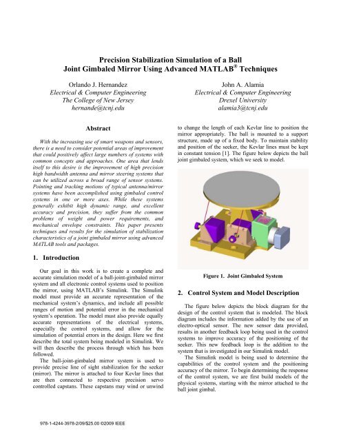
to change the length of each Kevlar line to position the
mirror appropriately. The ball is mounted to a support
structure, made up of a fixed body. To maintain stability
and position of the seeker, the Kevlar lines must be kept
in constant tension [1]. The figure below depicts the ball
joint gimbaled system, which we seek to model.
1. Introduction
Our goal in this work is to create a complete and
accurate simulation model of a ball-joint-gimbaled mirror
system and all electronic control systems used to position
the mirror, using MATLAB’s Simulink. The Simulink
model must provide an accurate representation of the
mechanical system’s dynamics, and include all possible
ranges of motion and potential error in the mechanical
system’s operation. The model must also provide equally
accurate representations of the electrical systems,
especially the control systems, and allow for the
simulation of potential errors in the design. Here we first
describe the total system being modeled in Simulink. We
will then describe the process through which has been
followed.
The ball-joint-gimbaled mirror system is used to
provide precise line of sight stabilization for the seeker
(mirror). The mirror is attached to four Kevlar lines that
are then connected to respective precision servo
controlled capstans. These capstans may wind or unwind
Figure 1. Joint Gimbaled System
2. Control System and Model Description
The figure below depicts the block diagram for the
design of the control system that is modeled. The block
diagram includes the information added by the use of an
electro-optical sensor. The new sensor data provided,
results in another feedback loop being used in the control
systems to improve accuracy of the positioning of the
seeker. This new feedback loop is the addition to the
system that is investigated in our Simulink model.
The Simulink model is being used to determine the
capabilities of the control system and the positioning
accuracy of the mirror. To begin determining the response
of the control system, we are first build models of the
physical systems, starting with the mirror attached to the
ball joint gimbal.
978-1-4244-3978-2/09/$25.00 ©2009 IEEE

Figure 2. Block Diagram of Control Systems and
Motor Control
The ball-joint gimbal mirror Simulink model has been
divided into four main systems, the digital signal
processing, servo-capstan operation, the Kevlar rope
behavior, and mirror’s physical behavior. The digital
signal processing model calculates the final length of the
Kevlar ropes for a given desired mirror orientation. The
Simulink blocks used in this system can be seen in the
figure below.
The calculation to determine the final length of the
Kevlar ropes is done by first converting the angles that
have been entered as the input to a direction cosine matrix.
The angles entered must be given in radians for the
direction cosine matrix to be properly calculated. The
direction cosine matrix provides a complete mathematical
description of the mirror’s orientation. The direction
cosine matrix is then operated on to determine the
location of the holes in the mirror to which the Kevlar
ropes are attached. The current coordinates of the hole in
the mirror’s new orientation is determined by multiplying
the direction cosine matrix with a diagonal matrix
containing the initial coordinates of the hole. This process
is summarized by the equations below where the first
matrix is the direction cosine matrix, and the second is a
diagonal matrix of the holes’ initial coordinates.
Figure 3. Simulink System Used to Calculate Final Rope Length
To determine the final coordinates of the hole in the
mirror each row must be summed, producing the X, Y,
and Z coordinates in the first, second and third rows
respectively. The initial positions of the holes are
determined from a Pro/Engineer model of the ball-joint
gimbal mirror at 0 degrees azimuth and 0 degrees
elevation. The coordinates where the rope meets the
capstan, also determined from the Pro/Engineer model of
the ball-joint gimbal mirror, is then subtracted from the
coordinates calculated previously. The magnitude of this
vector is then calculated to produce the distance between
the two points, giving us our final rope length. To avoid
initialization of the rope lengths, which may be seen as a
large disturbance by the system, the initial length of the
rope is subtracted from the commanded position, yielding
the change in rope length from the initial position as the
command received by the control system.
To determine the lengths of the ropes from the optical
encoders in the capstans we use the measure of the angle
provided and multiply it by the radius of the capstan. This
yields the length of rope that has been wound, or in the
case of a negative angle, unwound, from the capstan.
There is also no initialization added to the optical encoder,
resulting in the output being the change in rope length
from the initial position’s appropriate rope lengths.
⎡uˆ
⎢
⎢
uˆ
⎢⎣
uˆ
x
y
z
vˆ
x
vˆ
y
vˆ
z
wˆ
x ⎤ ⎡X
i
wˆ
⎥
×
⎢
y
⎥ ⎢
0
wˆ
⎥⎦
⎢
z ⎣ 0
0
Y
i
0
0 ⎤ ⎡X
⎢
0
⎥
⎥
= ⎢ Y
Z ⎥⎦
⎢
i ⎣ Z
xx
yx
zx
X
Y
Z
xy
yy
zy
X
X
Z
xz
yz
zz
⎤
⎥
⎥
⎥
⎦
(1)
The information from the optical controller is dealt
with in the same fashion as the input command. The
angles measured by the sensor are first converted to a
direction cosine matrix, and then through the calculations
previously mentioned the lengths of the ropes are
calculated and sent to the control system, which can be
seen in Figure 4.
The resulting signal from the control system is sent to
the servomotor-capstan system. The servomotor accepts
the signal and uses a lookup table to determine the
position the command given by the digital signal

processing system, corresponds to. The position is then
used to supply the electrical model of the servomotor with
a voltage proportional to the difference in current position
and commanded position. The Simulink blocks used to
create the model of the servomotor can be seen in Figure
5. The model of the servomotor assumes that the servo is
powered by a 5-volt source whose polarity may be
reversed to spin the servomotor in the opposite direction.
Figure 4. Simulink Model of Control System
Figure 5. Simulink Model of a Servo Motor
The mechanical components of the servomotor are
modeled as a rotating mass with a torque proportional to
the current through the electrical model. The angles of the
servomotor, as well as the current through the electrical
model, are sent to analog to digital converters, and the
torque is sent to the Kevlar rope system of the model.
The torque of the capstan is converted to a force vector
applied to the mirror. The force vector is calculated by
determining the unit vector, which points from the
capstan to the hole on the mirror to which the rope is
attached. The magnitude of the torque is then multiplied
through the unit vector, resulting in the appropriate force
vector, which is then passed to the mechanical model of
the mirror. The calculation of the force vector can be seen
in Figure 6. The calculation of the force vector in Figure 6
assumes that there is no change in the length of the rope
while under tension and that the line never becomes slack.
The three force vectors calculated through this fashion
are applied to the mechanical model of the mirror, which
can be seen in Figure 7. The model applies the forces at
the appropriate point on the mirror, which is mounted on
a spherical joint. The mirror is modeled as a body placed
on top of a spherical joint that is connected to an object
fixed in space.

Figure 6. Conversion of Capstan Torque to Force Vector
Figure 7. SimMechanics Physical Model of Mirror and Ball Joint Gimbal
3. Simulations and Results
A simulation was created to obtain data to compare the
behavior of the servomotors alone, both with and without
the optical sensor. Through this simulation, we are able to
infer the approximate benefits of the optical sensor. To
make the comparison eight simulations were created to
allow for comparison in both time and frequency domain
responses. The first four simulations are time domain
representations, first a step response, followed by a step
response that is then moved to a second position before
returning to its initial position. In both of these cases the

simulation was run with and without the optical sensor,
yielding the four time domain simulations. The next four
simulations were done in the frequency domain yielding
the frequency response of the servo system under the four
conditions used in the time domain analysis.
In the simulations involving the optical sensor, as
depicted below, the inaccuracy of the optical sensor was
used to calculated the expected steady state error, which
was then added into the model in the same fashion as the
steady state error previously expected according to the
measured results. The steady state error of the servo was
calculated by determining the inaccuracy the servomotor
experience because of the inaccuracy in mirror position
measurement.
Figure 8. Control System Block of Servo Simulink Model
Using this model, we were able to produce the results
previously mentioned. The first is the time domain step
response of the servomotor without the optical device.
This can be seen below, where the top graph is the
position, and the bottom graph is the error in position.
The next simulation uses the optical sensor. The
resulting graphs may be seen in Figure 10. When the
optical sensor is added the steady state error shrinks to
approximately 50μradians, compared to the 400μradians
seen in the simulation seen previously in Figure 9.
Figure 9. Step Response of Servo without Optical Sensor

Figure 10. Step Response of Servo with Optical Sensor
Figure 11. Double Step Response of Servo with Optical Sensor
4. Conclusions
The simulation results of both the time domain and
frequency domain support the expected results. The
relative benefits shown in the servomotor control will be
seen in the total system. The addition of the optical sensor
greatly improves the steady state error, as well as
bandwidth and magnitude responses. The simulation
model also allows the optical sensor accuracy to be
altered to different specifications in the future.
5. Acknowledgements
This work was accomplished thanks to the financial
support of a grant from the US Navy Naval Air Warfare
Center Weapons Division STTR grant N07-T007 under
Contract Number: N00014-07-M-0446.
6. References
[1] Christison, Donald, et al; Ball Joint Gimbal System, US
Patent 6396233, Issued May 28, 2002.