2001 - Volume 2 - Journal of Engineered Fibers and Fabrics

element basis, the Galerkin method requires
(28)
(38)
It is emphasized that this integral applies to a typical element
e and the integration is to be performed over the area A e
of the element. After the Green-Gauss theorem, the second
kind of heat influx, and the third kind of convection boundary
conditions are applied, and we may get the following equation:
The Equation (29) is an unsteady heat transfer problem
which may also be referred to as a transient or time-dependent
problem. Since the time variable t enters into such a
problem we can use the partial discretization to separate the
space variables and the time variable. The unknown temperature
parameter function T within a typical element e can be
written as follows:
Here the N(x, y) is the shape function vector and d e is the
vector of the nodal temperatures for element e. It follows that
Equation (29) may be written as follows:
where
(29)
(30)
(31)
(32)
The element capacitance matrix is defined by,
(39)
(40)
Then the following element matrices K xxe ,K yye ,K cve ,f cve ,
f q*e ,f qe
, and C e can be calculated [19, 24]. The global stiffness
matrix K, capacitance matrix C, and the nodal force vector
f can be assembled from these element matrices and the
local destination array.
The Enforcement of the Essential Boundary
Conditions
In the boundary conditions mentioned earlier, there is a
kind of condition that has constant temperatures at these
boundaries. These constant temperature boundary conditions
must be enforced before the global matrices can be used to
solve the unknown temperatures. In the programs coded for
this research the above boundary conditions are enforced by
a method which is based on the concept of penalty functions
[24]. This method is easy to apply and understand.
After the application of the essential boundary conditions
we get the following global matrices: K a ,C a , and f a . Here the
superscript ( a ) is used to indicate the assemblage matrices
after the application of the essential boundary conditions.
Then we get the following equation to solve
(41)
Equation (41) needs to be solved for the nodal temperature
as a function of time. There are different schemes to solve this
equation. They may be summarized in one convenient equation
as follows:
(42)
The element stiffness matrices are in turn given by,
y
and the element nodal force vectors by,
44 INJ Summer 2001
(33)
(34)
(35)
(36)
(37)
where the parameter q takes on values of 0, 1/2 and 1 for
the forward, central, and backward difference schemes,
respectively. The value 2/3 is for the Galerkin method [24]
and q = 2/3 is particularly useful because it is more accurate
than the backward difference scheme (q =1) and more stable
than the central difference scheme (q = 1/2). So q = 2/3 is
used in the calculation.
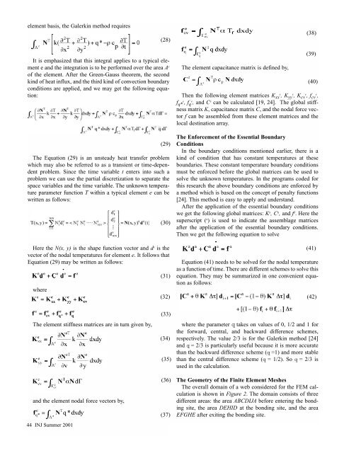
The Geometry of the Finite Element Meshes
The overall domain of a web considered for the FEM calculation
is shown in Figure 2. The domain consists of three
different areas: the area ABCDIJA before entering the bonding
site, the area DEHID at the bonding site, and the area
EFGHE after exiting the bonding site.