Graphics in LATEX using TikZ - TUG

Graphics in L A TEX using TikZ
Zofia Walczak
Faculty of Mathematics and Computer Science, University of Lodz
zofiawal (at) math dot uni dot lodz dot pl
Abstract
In this paper we explain some of the basic and also more advanced features of
the PGF system, just enough for beginners. To make our drawing easier, we use
TikZ, which is a frontend layer for PGF.
1 Introduction
In this paper we explain some of the basic and also
more advanced features of the PGF system, just
enough for beginners. To make our drawing easier,
we use TikZ, which is a frontend layer for PGF. The
commands and syntax of TikZ were influenced by
such sources as METAFONT, PSTricks, and others.
For specifying points and coordinates TikZ provides
a special syntax. The simplest way is to use
two TEX dimensions separated by commas in round
brackets, for example (3pt,10pt). If the unit is not
specified, the default values of PGF’s xy-coordinate
system are used. This means that the unit x-vector
goes 1 cm to the right and the unit y-vector goes
1 cm upward. We can also specify a point in the polar
coordinate system like this: (30:1cm); this means
“go 1 cm in the direction of 30 degrees”.
To create a picture means to draw a series of
straight or curved lines. Using TikZ we can specify
paths with syntax taken from MetaPost.
2 Getting started
First we have to set up our environment. To begin
with, we set up our file as follows:
\documentclass{article}
\usepackage{tikz}
\begin{document}
Document itself
\end{document}
Then we start to create pictures. The basic building
block of all the pictures in TikZ is the path.
You start a path by specifying the coordinates of
the start point, as in (0, 0), and then add a “path
extension operation”. The simplest one is just --.
The operation is then followed by the next coordinate.
Every path must end with a semicolon. For
drawing the path, we use \draw command which is
an abbreviation for \path[draw]. The \filldraw
command is an abbreviation for \path[fill,draw].
The rule is that all TikZ graphic drawing commands
must occur as an argument of the \tikz command
or inside a {tikzpicture} environment. The
L A TEX version of the {tikzpicture} environment is:
\begin{tikzpicture}[]
\end{tikzpicture}
All options given inside the environment will
apply to the whole picture.
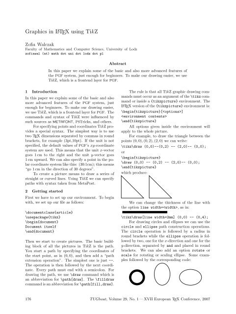
For example, to draw the triangle between the
points (0, 0), (0, 2), (2, 0) we can write:
\tikz\draw (0,0)--(0,2) -- (2,0)-- (0,0);
or
\begin{tikzpicture}
\draw (0,0) -- (0,2) -- (2,0)-- (0,0);
\end{tikzpicture}
which produce:
We can change the thickness of the line with
the option line width=, as in:
\tikz\draw[line width=2mm] (0,0) -- (0,4);
For drawing circles and ellipses we can use the
circle and ellipse path construction operations.
The circle operation is followed by a radius in
round brackets while the ellipse operation is followed
by two, one for the x-direction and one for the
y-direction, separated by and and placed in round
brackets. We can also add an option rotate or
scale for rotating or scaling ellipse. Some examples
followed by the corresponding code:
176 TUGboat, Volume 29, No. 1 — XVII European TEX Conference, 2007

Graphics in L A TEX using TikZ
\tikz\draw[line width=2mm] (0,0)
circle (4ex);
\tikz\draw (0,0) ellipse (20pt and 28pt);
\tikz\draw (0,0) ellipse (28pt and 20pt);
\tikz\draw[rotate=45] (0,0)
ellipse (16pt and 20pt);
\tikz\draw[scale=1.5,rotate=75] (0,0)
ellipse (10pt and 16pt);
We also have the rectangle path construction operation
for drawing rectangles and grid, parabola,
sin, cos and arc as well. Below are examples of
using these constructions.
\begin{tikzpicture}
\draw[step=.25cm,gray,thick]
(-1,-1) grid (1,1);
\end{tikzpicture}
\begin{tikzpicture}
\draw (-.5,0)--(1.5,0);
\draw (0,-.5)--(0,1.5);
\draw (1,0) arc (-25:70:1cm);
\end{tikzpicture}
\tikz\draw (0,0) arc (0:180:1cm);
\tikz \draw[fill=gray!50] (4,0)-- +(30:1cm)
arc (30:60:1cm) -- cycle;
\tikz \draw[fill=gray!50] (4,0)-- +(30:2cm)
arc (30:60:1cm) -- cycle;
There is a very useful command \tikzstyle
which can be used inside or outside the picture environment.
With it we can set up options, which
will be helpful in drawing pictures. The syntax of
this command is
\tikzstyle+=[]
We can use it as many times as we need. It is possible
to build hierarchies of styles, but you should
not create cyclic dependencies. We can also redefine
existing styles, as is shown below for the predefined
style help lines:
\begin{tikzpicture}
\draw (-1.5,0) -- (1.5,0);
\draw (0,-1.5) -- (0,1.5);
\draw (0,0) circle (.8cm);
\draw (-1,-1) rectangle (1,1);
\draw[gray] (-.5,-.5) parabola (1,1);
\end{tikzpicture}
The arc path construction operation is useful
for drawing the arc for an angle. It draws the part of
a circle of the given radius between the given angles.
This operation must be followed by a triple in round
brackets. The components are separated by colons.
The first and second are degrees on the circle and
the third is its radius. For example, (20 : 45 : 2cm)
means that it will be an arc from 20 to 45 degrees
on a circle of radius 2 cm.
\tikzstyle{my help lines}=[gray,
thick,dashed]
\begin{tikzpicture}
\draw (0,0) grid (2,2);
\draw[style=my help lines] (2,0)
grid +(2,2);
\end{tikzpicture}
If the optional + is given, it means that the new
options are added to the existing definition. It is also
possible to set a style using an option
just after opening the tikzpicture environment.
When we want to apply graphic parameters to
only some path drawing or filling commands we can
use the scope environment.
TUGboat, Volume 29, No. 1 — XVII European TEX Conference, 2007 177

Zofia Walczak
4 Adding text to the picture
For adding text to the picture we have to add node
to the path specification, as in the following:
B
B
A
B
A
A
D
C
\begin{tikzpicture}
\begin{scope}[very thick,dashed]
\draw (0,0) circle (.5cm);
\draw (0,0) circle (1cm);
\end{scope}
\draw[thin] (0,0) circle (1.5cm);
\end{tikzpicture}
3 Filling with color
Using command \fill[color] we can fill with the
given color a domain bounded by any closed curve.
For closing the current path we can use -- cycle.
For the color argument, we can use either name of
color, for example green, white, red, or we can mix
colors together as in green!20!white, meaning that
we will have 20% of green and 80% of white mixed.
\tikz\draw (1,1) node{A} -- (2,2) node{B};
\tikz\draw (1,1) node[circle,draw]{A} --
(2,2) node[circle,draw]{B};
\tikz\draw (0,0) node{D} -- (2,0) node{C}
-- (2,1) node{B} -- (0,1) node{A} --cycle;
Nodes are inserted at the current position of the
path (points A and B in the first example); the option
[circle,draw] surrounds the text by a circle,
drawn at the current position (second example).
Sometimes we would like to have the node to
the right or above the actual coordinate. This can
be done with PGF’s so-called anchoring mechanism.
Here’s an example:
B
A
\begin{tikzpicture}
\draw (-.5,0)--(1.5,0);
\draw (0,-.5)--(0,1.5);
\fill[gray] (0,0) -- (1,0) arc (0:45:1cm)
-- cycle;
\end{tikzpicture}
\tikz\draw[line width=2mm,color=gray]
(0,0) circle (4ex);
\qquad
\tikz\draw[fill=gray!30!white] (0,0)
ellipse (20pt and 28pt);
\qquad
\tikz\draw[fill=gray!60!white] (0,0)
ellipse (28pt and 20pt);
\begin{tikzpicture}
\draw (1,1) node[anchor=north east,circle,
draw]{A} -- (2,2) node[anchor=south west,
circle,draw]{B};
\end{tikzpicture}
This mechanism gives us very fine control over the
node placement.
For placing simple nodes we can use the label
and the pin option. The label option syntax is:
label=[]:
Top
My rectangle
Bottom
\tikz \node[rectangle,draw,
label=above:Top,label=below:
Bottom]{my rectangle};
When the option label is added to a node operation,
an extra node will be added to a path containing
. It is also possible to specify the label
distance parameter, which is the distance additionally
inserted between the main node and the label
node. The default is 0 pt.
178 TUGboat, Volume 29, No. 1 — XVII European TEX Conference, 2007

Graphics in L A TEX using TikZ
9
12
clock
6
3
12
\tikz[label distance=2mm]
\node[circle,fill=gray!45,
label=above:12,label=right:3,
label=below:6,label=left:9]{clock};
9
The pin option is similar to the label option
but it also adds an edge from this extra node to the
main node. The syntax is as follows:
pin=[]:{text}.
pin distance is an option which must be given
as part of the \tikz command. The default is 3 ex.
A
example
\tikz[pin distance=4mm]
\draw (1,1) node[circle,fill=gray!45,
pin=above:12,pin= right:3,pin=below:6,
pin=left:9]{} circle (1cm);
B
5 The plot operation
If we have to append a line or curve to a path that
goes through the large number of coordinates, we
can use the plot operation. There are two versions
of plot syntax: --plot and
plot .
The first plots the curve through the coordinates
specified in ; the second
plots the curve by first ”moving” to the first coordinate
of the curve. The following example shows
the difference between --plot and plot.
6
9
3
12
\tikz\draw (0,1) -- (1,1) --plot
coordinates {(2,0) (2,1.5)};
\tikz\draw[color=gray] (0,1) -- (1,1)
plot coordinates {(2,0) (2,1.5)};
6
3
6 Plotting functions
For plotting functions we have to generate many
points and for that TEX has not enough computational
power, but it can call external programs that
can easily produce the necessary points. TikZ knows
how to call Gnuplot. In this case, the plot operation
has the following syntax:
plot[id=] function{formula}.
When TikZ encounters this operation, it will
create a file called .gnuplot, where
by default is the name of the .tex file. It
is not strictly necessary to specify an , but it
is better when each plot has its own unique .
Next TikZ writes some initialization code into this
file. This code sets up things such as the plot operation
writing the coordinates into another file, named
.table.
y
\begin{tikzpicture}[domain=0:2]
\draw[thick,color=gray,step=.5cm,
dashed] (-0.5,-.5) grid (3,3);
\draw[->] (-1,0) -- (3.5,0)
node[below right] {$x$};
\draw[->] (0,-1) -- (0,3.5)
node[left] {$y$};
\draw plot[id=x] function{x*x};
\end{tikzpicture}
The option samples= sets the number of
samples used in the plot (default is 25) and the
option domain=: sets the domain between
which the samples are taken.
If you want to use the plotting mechanism you
have to be sure that the gnuplot program is installed
on your computer, and TEX is allowed to call
external programs.
References
[1] Till Tantau, The TikZ and PGF Packages,
Manual for ver. 1.09, http://sourceforge.
net/projects/pgf
x
TUGboat, Volume 29, No. 1 — XVII European TEX Conference, 2007 179