SIMSCRIPT II.5 Programming Language

process AIRPLANE
call TOWER giving GATE yielding RUNWAY
work TAXI.TIME (GATE, RUNWAY) minutes
request 1 RUNWAY
work TAKEOFF.TIME (AIRPLANE) minutes
relinquish 1 RUNWAY
end " process AIRPLANE
process AIRPLANE
call TOWER giving GATE yielding RUNWAY
work TAXI.TIME (GATE, RUNWAY) minutes
request 1 RUNWAY
Since
S1962
Programming Language

Copyright © 1997 CACI Products Co.
September 1997
All rights reserved. No part of this publication may be reproduced by any means without written permission from CACI.
For product information or technical support contact:
In the US and Pacific Rim:
In Europe:
CACI Products Company
CACI Products Division
3333 North Torrey Pines Court Coliseum Business Centre
La Jolla, California 92037
Riverside Way, Camberley
Phone: (619) 824.5200
Surrey GU15 3YL UK
Fax: (619) 457.1184 Phone: +44 (0) 1276.671.671
Fax: +44 (0) 1276.670.677
The information in this publication is believed to be accurate in all respects. However, CACI cannot assume
the responsibility for any consequences resulting from the use thereof. The information contained herein is
subject to change. Revisions to this publication or new editions of it may be issued to incorporate such change.
SIMGRAPHICS I, SIMGRAPHICS II and SIMSCRIPT II.5 are registered trademarks of CACI Products Company.
Windows is a registered trademark of Microsoft Corporation.

Table of Contents
Preface ................................................................................................................ a
1. SIMSCRIPT II.5 BASIC CONCEPTS ................................................................... 1
1.1 INTRODUCTION........................................................................................... 1
1.2 VARIABLES ................................................................................................ 1
1.3 READING INPUT DATA ................................................................................ 2
1.4 CONSTANTS ............................................................................................... 3
1.5 ARITHMETIC EXPRESSIONS ......................................................................... 4
1.6 COMPUTING VARIABLE VALUES ................................................................. 5
1.7 SPECIALIZED COMPUTATION STATEMENTS .................................................. 6
1.8 DISPLAYING THE RESULTS OF COMPUTATION .............................................. 6
1.9 SKIPPING UNWANTED INPUT DATA .............................................................. 9
1.10 LOGICAL EXPRESSIONS .......................................................................... 10
1.11 CHANGING THE FLOW OF COMPUTATION USING LOGICAL EXPRESSIONS .. 12
1.12 MORE ON LOGICAL EXPRESSIONS .......................................................... 16
1.13 REPETITION USING CONTROL PHRASES................................................... 19
1.14 CONTROL PHRASES EXTENDED TO COVER MORE THAN ONE STATEMENT 21
1.15 LOGICAL CONTROL PHRASES ................................................................. 22
1.16 ALTERING THE FLOW OF CONTROL WITHIN A LOOP................................. 26
1.17 CHANGING THE FLOW OF CONTROL BY DIRECT ORDER .......................... 27
1.18 THE LOGICAL END OF A PROGRAM ......................................................... 29
1.19 THE PHYSICAL END OF A PROGRAM ....................................................... 29
1.20 A NOTE ON SIMSCRIPT II.5 PROGRAM FORM ....................................... 29
1.21 CLARIFYING COMMENTS IN A PROGRAM ................................................. 30
1.22 SOME SAMPLE SIMSCRIPT II.5 LEVEL 1 PROGRAMS ............................ 31
1.22.1 Roots of a Quadratic Expression .....................................................................31
1.22.2 Finding the Area of a Triangle ..........................................................................32
1.22.3 Finding the Maximum and Minimum of a Set of Numbers ...............................33
1.22.4 Computing Square Roots .................................................................................34
2. PROGRAMMING LANGUAGE CONCEPTS ............................................................ 37
2.1 VARIABLE AND LABEL NAMES REVISITED ................................................. 37
2.2 VARIABLE MODES ................................................................................... 37
2.2.1 REAL and INTEGER Variables .........................................................................38
2.3 EXPRESSION MODES ............................................................................... 40
2.4 SYSTEM-DEFINED CONSTANTS ................................................................. 42
2.5 SUBSCRIPTED VARIABLES ........................................................................ 43
2.6 READING SUBSCRIPTED VARIABLES.......................................................... 49
2.7 USING SUBSCRIPTED VARIABLES IN EXPRESSIONS .................................... 50
2.8 NESTED DO LOOPS ................................................................................. 51
2.9 THE STRUCTURE OF A SIMSCRIPT II.5 PROGRAM ................................... 51
2.10 ROUTINE DEFINITION ............................................................................. 54
2.11 GLOBAL AND LOCAL VARIABLES ............................................................. 56
2.12 ROUTINE ARGUMENTS ........................................................................... 60
2.13 ROUTINES USED AS FUNCTIONS ............................................................. 62
2.14 GLOBAL AND LOCAL VARIABLES, ROUTINES, FUNCTIONS, AND SIDE
EFFECTS .............................................................................................. 64
i

SIMSCRIPT II.5 Programming Language
2.15 LIBRARY FUNCTIONS ...............................................................................64
2.16 USING NON-SIMSCRIPT ROUTINES ....................................................... 65
2.17 RETURNING RESERVED ARRAYS TO FREE STORAGE ............................... 65
2.18 ARRAY POINTERS AS ROUTINE ARGUMENTS ............................................66
2.19 TEXT MODE VARIABLES ......................................................................... 69
2.20 READING AND DISPLAYING TEXT VARIABLES............................................ 70
2.21 OPERATIONS WITH TEXT VARIABLES .......................................................71
2.21.1 Concatenation: CONCAT.F(text1, text2...textn)...............................................72
2.21.2 Substring: SUBSTR.F(text, index, length) .......................................................72
2.21.3 Pattern Matching: MATCH.F(text, pattern, skip) ............................................. 73
2.21.4 Length Function: LENGTH.F(text) ..................................................................73
2.21.5 Case Conversion: UPPER.F(text) and LOWER.F(text) .................................. 73
2.21.6 String Repetition: REPEAT.F(string,count)...................................................... 73
2.21.7 Truncation and Expansion: FIXED.F(string,length) .........................................73
2.21.8 Blank Character Elimination: TRIM.F(string, flag)........................................... 74
2.21.9 INTEGER to TEXT Conversion ITOT.F(integer)............................................ 74
2.22 ALPHA VARIABLES ..................................................................................74
2.22.1 TEXT to ALPHA Conversion: TTOA.F(text) ....................................................75
2.22.2 ALPHA to TEXT Conversion: ATOT.F(alpha) .................................................75
2.23 RECURSIVE ROUTINES ............................................................................75
2.24 PRE-PROCESSING PROGRAM TEXT .........................................................81
2.25 MORE ON CHANGING THE FLOW OF COMPUTATION..................................84
2.26 SOME DATA-RELATED LOGICAL VALUES ..................................................86
2.27 MORE SAMPLE SIMSCRIPT II.5 LEVEL 1 PROGRAMS ............................. 89
2.27.1 A Data Analysis Program: 1 .............................................................................89
2.27.2 A Data Analysis Program: 2............................................................................. 90
2.27.3 A Matrix Multiplication Program ........................................................................91
2.27.4 A Matrix Multiplication Routine .........................................................................92
2.28 MORE ON PROGRAM FORMAT ................................................................. 93
2.29 A USEFUL OUTPUT STATEMENT ..............................................................94
2.30 SUBPROGRAM VARIABLES .......................................................................95
2.31 THE STORE STATEMENT .........................................................................98
3. Input/Output Concepts................................................................................ 99
3.1 INTRODUCTION ......................................................................................... 99
3.2 A SEARCH CAPABILITY.............................................................................. 99
3.3 A STATEMENT FOR COMPUTING SOME STANDARD FUNCTIONS OF
VARIABLES .............................................................................................100
3.4 INPUT/OUTPUT STATEMENTS ..................................................................103
3.4.1 Physical Device Specification ..........................................................................104
3.4.2 The Formatted I/O Statements READ and Write .............................................106
3.4.3 Format Lists .....................................................................................................110
3.4.4 Controlled READ and WRITE Statements ......................................................116
3.4.5 Variable Formats.............................................................................................. 117
3.5 MISCELLANEOUS INPUT/OUTPUT STATEMENTS AND FACILITIES .................119
3.5.1 Logical File Assignment: The OPEN Statement ..............................................119
3.5.2 End-of-File Conditions .....................................................................................120
ii

Contents
3.5.3 Repositioning Files ............................................................................................121
3.5.4 Input/Output of Nondecimal Information ...........................................................121
3.6 INTERNAL EDITING OF DATA ................................................................... 122
3.7 WRITING FORMATTED REPORTS ............................................................ 124
3.7.1 Page Heading Control .......................................................................................136
4. MODELLING CONCEPTS................................................................................. 137
4.1 INTRODUCTION ....................................................................................... 137
4.2 ENTITIES AND ATTRIBUTES ..................................................................... 137
4.3 SETS ..................................................................................................... 139
4.4 TEMPORARY ENTITIES ............................................................................ 144
4.5 PERMANENT ENTITIES ............................................................................ 147
4.6 SYSTEM ATTRIBUTES ............................................................................. 149
4.7 ATTRIBUTE DEFINITIONS: MODE AND DIMENSIONALITY ........................... 150
4.8 SETS: THEIR DECLARATION AND USE ...................................................... 151
4.9 ENTITY CONTROL PHRASES ................................................................... 164
4.10 COMMON ATTRIBUTES .......................................................................... 168
4.11 COMPOUND ENTITIES ............................................................................ 170
4.12 IMPLIED SUBSCRIPTS ............................................................................ 172
4.13 DISPLAYING ATTRIBUTE VALUES ............................................................ 174
4.14 SOME SAMPLE PROGRAMS ................................................................... 176
4.14.1 An Inventory Control Example ....................................................................... 176
4.14.2 A Data Analysis Application ...........................................................................178
4.14.3 An Analysis of Prime Numbers ......................................................................181
4.14.4 Dynamic Definition and Use of Attributes .......................................................181
5. DISCRETE SIMULATION CONCEPTS ................................................................ 183
5.1 INTRODUCTION ....................................................................................... 183
5.2 DESCRIBING A SYSTEM MODEL .............................................................. 183
5.2.1 Event Declaration............................................................................................. 187
5.2.2 Event Notices ...................................................................................................188
5.2.3 Process Declaration .........................................................................................189
5.2.4 Scheduling Events and Processes ..................................................................190
5.2.5 Processes and Events Scheduled for the Same Time .....................................191
5.3 THE SIMULATION MECHANISM ................................................................ 193
5.3.1 The Simulation Clock .......................................................................................195
5.3.2 Assigning Event and Process Attributes ..........................................................197
5.3.3 Process Interactions ........................................................................................ 200
5.3.4 Interrupting and Resuming a Process ..............................................................201
5.3.5 Processes and Resources ...............................................................................202
5.3.6 Requesting and Relinquishing Resources ....................................................... 203
5.3.7 Process Notice: Additional Attributes ..............................................................205
5.3.8 External Processes and Events ....................................................................... 207
5.3.9 Triggering Processes and Events Externally ...................................................209
5.3.10 Time and Date Expressions in External Data .................................................210
5.4 MODELLING STATISTICAL PHENOMENA .................................................... 214
5.4.1 Random Step Variables ...................................................................................220
5.4.2 Random Linear Variables ................................................................................ 220
5.4.3 Programmer-Defined Random Variables......................................................... 221
iii

SIMSCRIPT II.5 Programming Language
5.5 SIMULATION ANALYSIS ............................................................................ 223
5.6 MODEL VERIFICATION AND DEBUGGING ................................................... 232
5.7 SYNCHRONOUS VARIABLES .....................................................................236
5.8 SIMULATION EXAMPLE ............................................................................ 238
5.8.1 A Sample Model................................................................................................ 238
6. ADVANCED TOPICS........................................................................................ 249
6.1 INTRODUCTION ....................................................................................... 249
6.2 PROGRAMMER-DEFINED ARRAY STRUCTURES: POINTER VARIABLES .......249
6.3 STILL MORE ON CHANGING THE FLOW OF COMPUTATION .........................257
6.4 ATTRIBUTE DEFINITIONS: PACKING AND EQUIVALENCE ............................260
6.5 ATTRIBUTE DEFINITIONS: FUNCTIONS ......................................................271
6.6 COMPOUND ENTITIES INVOLVING TEMPORARY ENTITIES........................... 272
6.7 TWO ILLUSTRATIONS OF SET RANKING BY FUNCTION ATTRIBUTES ...........273
6.8 USING “OPTIONAL” ATTRIBUTES ...............................................................275
6.9 DELETION OF SET ROUTINES ................................................................. 278
6.10 LEFT-HANDED FUNCTIONS .....................................................................279
6.11 MONITORED VARIABLES .........................................................................282
6.12 IMPLEMENTATION DETAILS FOR THE TALLY STATEMENT .........................288
APPENDIX A. FORMAT CONVENTIONS USED IN PRINT STATMENTS...................... 291
APPENDIX B.FUNCTIONS AND ROUTINES .............................................................295
B.1 FUNCTIONS .................................................................................................295
B.2. ROUTINES ..................................................................................................305
APPENDIX C. SIMSCRIPT REFERENCE SYNTAX ................................................ 307
C.1 BASIC CONSTRUCTS................................................................................... 307
C.2 Primitives ..................................................................................................308
C.3 Metavariables ...........................................................................................309
C.3 THE STATEMENT SYNTAX ........................................................................... 312
C.5 Preamble Statement Precedence Rules ..................................................330
Index..................................................................................................................333
iv

Figures
Figure 1-1. Flow of Control After an if Statement ............................................ 13
Figure 1-2. Flow of Control After Shortened if Statement ............................... 14
Figure 2-1. A List Structure: One-dimensional Array ....................................... 43
Figure 2-2. Elements of a One-dimentional Array Called LIST ....................... 44
Figure 2-3. A Table Structure: A Two-dimensional Array ................................ 45
Figure 2-4. Elements of a Two-dimensional Array Called TABLE .................. 45
Figure 2-5a. Program Consisting of a Subprogram Called by a Main Routine . 53
Figure 2-5b. Program Consisting of Two Subprograms Called by a
Main Routine ................................................................................. 53
Figure 2-5c. Program Consisting of Three Subprograms and a Main Routine 54
Figure 2-6. Tree Construction ......................................................................... 79
Figure 2-7. A Binary Tree ................................................................................ 80
Figure 2-8. A Complex Tree ............................................................................ 81
Figure 3-1. Report Using Row and Column Repetition ................................. 125
Figure 3-2. Column Repetition, Page 1 ......................................................... 130
Figure 3-3. Column Repetition, Page 2 ......................................................... 131
Figure 3-4. An Example of Column Repetition .............................................. 132
Figure 3-5. An Example of Format Suppression ........................................... 134
Figure 4-1. Storage of Attributes in a Two-dimensional Array ...................... 138
Figure 4-2. Order of Storage of the Attributes of an Entity ............................ 139
Figure 4-3. Automatically-defined Attributes of COMMUNITY Entities ......... 140
Figure 4-4. Automatically-defined Attributes for Members of the Class MAN 140
Figure 4-5. Owner-member Set Relationships .............................................. 141
Figure 4-6. Set Relationships ........................................................................ 142
Figure 4-7. Set Relationships ........................................................................ 143
Figure 4-8. Entity Creation ............................................................................ 145
Figure 4-9. Attribute Storage of Permanent Entities ..................................... 148
Figure 4-10. Storage of Attributes of a Permanent Entity ............................. 152
Figure 4-11. Storage of Attributes of a Temporary Entity .............................. 152
Figure 4-12. Storage of System Attributes and Set Pointers ........................ 152
Figure 4-13. Entity Structures for FARM and DOG ....................................... 154
Figure 4-14. Entity Records .......................................................................... 155
Figure 4-15. Entity Records .......................................................................... 155
Figure 4-16. Entity Records .......................................................................... 157
Figure 4-17. Entity Records .......................................................................... 158
Figure 4-18. A Set with Two Members .......................................................... 159
Figure 4-19. A Set with Three Members ....................................................... 160
Figure 4-20. FIFO and LIFO Set Organizations ............................................ 163
Figure 4-21. Entity Structures for TANKER and TUG ................................... 170
Figure 4-22. Display of Result Produced by Data Analysis Program ............ 180
v

SIMSCRIPT II.5 Programming Language
Figure 5-1. An Activity Delimited by Two Events ...........................................184
Figure 5-2. A Process May Be Considered to be Comprised of a Sequence of
Events Occurring in Time .............................................................185
Figure 5-3a. Two Overlapping Activites ..........................................................186
Figure 5-3b. Two Nested Activities .................................................................187
Figure 5-3c. Two Activities with a Common Event Time .................................187
Figure 5-4. Possible Layout of Event Notice Entities .....................................189
Figure 5-5. The Future Events Set Organization ...........................................194
Figure 5-6. Attributes of Process Notices Created by Process Declarations
Above ...........................................................................................207
Figure 5-7. A Rectangular Coordinates System ............................................ 218
Figure 5-8. Storage of RANDVAR Sample Values .........................................223
Figure 6-1. One-dimensional Array X with Its Base Pointer ...........................250
Figure 6-2. Base Pointers in a Two-Dimensional Array .................................250
Figure 6-3. Base Pointers in a Three-Dimensional Array .............................. 251
Figure 6-4. Memory Structure After Reserve Statement ................................252
Figure 6-5. Memory Structure After Assignment of Data Arrays to Row
Pointers ........................................................................................ 253
Figure 6-6. Family Tree.................................................................................. 254
Figure 6-7. Family Tree Stored in a Rectangular Array .................................254
Figure 6-8. Family Tree Stored in a Ragged Table........................................ 254
Figure 6-9. Memory Structure for Family Tree, N = 4 ....................................256
Figure 6-10. Entity Storage ............................................................................264
Figure 6-11. Array Storage ............................................................................268
Figure 6-12. Array Storage ............................................................................ 268
Figure 6-13. Record Structure .......................................................................277
vi

Preface
SIMSCRIPT II.5 is a rich and versatile computer programming language enhanced with computer
graphics, designed to solve general programming problems. This book, which describes the
SIMSCRIPT II.5 language, is divided into chapters describing non-graphical language "levels"
which provide an organized path through the language:
Level 1 (Chapters 1 and 2): General purpose language statements.
Level 2 (Chapters 3 and 4): The entity-attribute-set features of SIMSCRIPT II.5. These features
have been updated and augmented to provide a more powerful list-processing capability.
This level also contains a number of new data types and programming features.
Level 3 (Chapter 5): The simulation-oriented part of SIMSCRIPT II.5, containing statements
for time advance, event-processing, generation of statistical variates, and accumulation and
analysis of simulation-generated data. The powerful new modeling constructs of processes and
resources are described in great detail.
Chapter 6 is a collection of various topics which need not be understood for initial use of
SIMSCRIPT II.5. This chapter also describes several features of the language which are obsolete,
but are being supported for compatibility.
A companion text, Building Simulation Models with SIMSCRIPT II.5, teaches the fundamentals of
simulation methodology through the use of SIMSCRIPT II.5 case studies. The material in this book
relates closely to the short course given regularly by the CACI Products Company.
A third book, SIMSCRIPT II.5 Reference Handbook, provides a description and examples of each
of the language elements in alphabetical order.
Interactive simulation graphics for SIMSCRIPT II.5 is described separately, in the SIMGRAPHICS
II User's Guide for SIMSCRIPT II.5. Other features of SIMSCRIPT II.5 are covered in the user's
manual for each specific system.
SIMSCRIPT II.5 is available for PCs running WindowsNT and Windows95. It is also available for
VMS systems and most UNIX workstations.
Free Trial Offer
SIMSCRIPT II.5 is available on a free trial basis. We provide everything needed for a complete
evaluation on your computer. There is no risk to you.
a

SIMSCRIPT II.5 Programming Language
Training Courses
Training courses in SIMSCRIPT II.5 are scheduled on a recurring basis in the following
locations:
La Jolla, California
Washington, D.C.
London, United Kingdom
On-site instruction is available. Contact CACI for details.
For information on free trials or training, please contact the following:
In the U.S. and Pacific Rim:
In the UK and Europe:
CACI Products Company
CACI Products Division
3333 North Torrey Pines Court Coliseum Business Centre
La Jolla, California 92037
Riverside Way, Camberley
(619) 824.5200 Surrey GU15 3YL UK
Fax: (619) 457.1184 +44 (0) 1276.671.671
Fax: +44 (0) 1276.670.677
b

1. SIMSCRIPT II.5 Basic Concepts
1.1 Introduction
A computer program is a list of instructions directing a computer to perform certain operations on
data. A programming language is used by a programmer to describe the data and the actions to be
performed. SIMSCRIPT II.5 is one such programming language. Here is a simple example of a
SIMSCRIPT II.5 program:
read X and Y
add X to Y
print 1 line with Y thus
The Sum is: *****
stop
This program consists of four SIMSCRIPT II.5 statements. The statements are instructions to:
1. Read the values of two variables called X and Y from input data
2. Add these variables together
3. Print the sum of the variables along with the explanatory message, The Sum is:, and
4. Stop.
The example illustrates the basic computer operations of input (reading data), computation (in this
case, addition), and output (printing results).
In program examples throughout this book, SIMSCRIPT words and commands will be printed in
lower case characters. Variable names, routine names, and other user-supplied terms will be printed
in upper case characters. Thus, in the above example, read, and, add, to, print, line,
with, thus, and stop are all SIMSCRIPT words. X, Y, and the phrase, The Sum is: are expressions
provided by the programmer. SIMSCRIPT words which appear in the text (apart from
those in program examples) will appear in bold characters. Again, variable names appear in upper
case characters. Finally, small segments of code are presented in the ‘courier’ font as shown
above.
Although SIMSCRIPT does support string variables, the rest of this chapter focuses on integers and
reals. See paragraph 2.19.
1.2 Variables
As shown in the above example, programs use identifying names to refer to values of program variables.
A variable is a data item that may take on different values as it is acted upon by operations.
A program statement such as:
add X to Y
1

SIMSCRIPT II.5 Programming Language
means add the current value of X to the current value of Y, giving Y a new value.
A variable identifying name is any combination of letters, digits, and periods that contains at least
one letter, so that it may be distinguished from a number. For example, X, COST,
ACCOUNTS.RECEIVABLE, SIZE, MAN3, PART1, 5Y, and 1A are all legal names, whereas 27,
1, and 4.6 are not. A slight restriction on variable naming is that any periods appearing as the last
characters of a name are completely ignored. Upper and lower case distinctions are also ignored.
Thus, Myvar, MyVar, and MYVAR all refer to the same quantity. It will be shown later in this
manual how this rule may be used as a notational aid.
Hereafter, whenever a variable name is used in a statement, it is understood to refer to the value of
the variable identified by that name, not to the name itself. The values given to numeric variables
may be whole numbers (integers) or numbers with a fractional part (decimal numbers). Thus, the
value associated with a variable named X may at various times be 0 or 125 or 16.72 or -0.00001,
or whatever number has most recently been assigned to X. The range in magnitude of numbers that
can be internally represented in a computer and the accuracy with which numbers can be represented
are, of course, subject to limits. These limits depend on the particular machine but, for the
present, may be taken to be sufficiently generous not to be the subject of concern.
At the start of program execution, the value of each numeric variable is set equal to zero. These
variables are said to be "initialized to zero."
1.3 Reading Input Data
One way in which specific numeric values can be assigned to program variables is by reading numbers
as input data. An example of the read statement is:
read X, Y and QUANTITY
X, Y, and QUANTITY are variable names. They are used in this statement in a variable name list.
In general, a SIMSCRIPT II.5 list consists of a string of quantities separated by either a comma, or
the word and, or a comma followed by the word and. Some examples of variable name lists as they
might appear in read statements are:
read PRICE, QUANTITY, DISCOUNT
read PLACE and DISTANCE
read NAME, DATE, PLACE and TIME
read NAME, and DATE, PLACE and TIME
The general form of a read statement is:
read variable name list
When a SIMSCRIPT program executes a read statement, it reads as many fields from the input
data as there are variable names listed in the statement. Successive numeric values are read and
2

SIMSCRIPT II.5 Basic Concepts
assigned to corresponding variables in the read list. The numbers can be entered in the input data
in integer or decimal form. For example, the numbers 5, 5.0, and 5.000 are equivalent.
Data items read into or printed by a computer are treated in physical groupings called records. Examples
of a record are a single line typed on a computer terminal, a record, or a line printed on a
printer. Within a record, data items are considered to be separated into fields. A field is a contiguous
string of symbols delimited at the beginning and the end by at least one blank. Numeric data
fields may also be delimited by the beginning or the end of a record. Each numeric value occupies
one data field.
Successive read statements do not necessarily read new input records, because a SIMSCRIPT II.5
program can treat input data as a continuous stream of data fields. The precise location, then, of a
number within a record is not considered. An example illustrates this "free-form" concept: Read
X, Y, Z sets X to the value 3, Y to the value 2.1, and Z to the value 67.33 when each of the sets
of input data records in table 1-1 is read.
Table 1-1. Sample Data Records
_______________________________________________________________________________
Record Number Values
(1) record 1 3.0 2.1 67.33
(2) record 1 3.00
record 2 2.1 67.33
(3) record 1 3
record 2 2.1
record 3 67.33
_______________________________________________________________________________
1.4 Constants
Program statements may use numbers directly, such as the "2" in add 2 to SUM, or the number
"3.14" in add 3.14 to VOLUME. These numbers are called constants. When used, they refer to
their literal values. They are not names of variables and do not represent other values.
Constants may have the same range of numeric values as variables, and where appropriate, may be
used interchangeably in all computations. Constants differ from variables in that their values cannot
be changed. Add 5 to X is a legal use of the variable X and the constant 5. Add 5 to 4 is not
a legal use of the constant 4 because it is giving a new value of 9 to the constant 4.
Whole numbers and fractional numbers, signed or unsigned, are allowed as constants. When equivalent
representations of a number exist, they have the same value; 2.5 and 002.500 both represent
the same number. The statements add 1 to COUNTER and add 1.00 to COUNTER have the
same effect.
3

SIMSCRIPT II.5 Programming Language
1.5 Arithmetic Expressions
Arithmetic expressions are formed by combining variables and constants with arithmetic operators.
The arithmetic operators are + (add), - (subtract), * (multiply), / (divide), and ** (exponentiate).
Two of these operators, plus and minus, can be used as unary operators, that is, with a single variable
or constant. The constants +1 and -1 are examples of the use of plus and minus as unary operators
on the constant 1. All of the operators can be used as binary operators, that is, with two
variables (or constants or a variable and constant). If we let A and B represent either a variable or a
constant, then + A and - A are examples of plus and minus as unary operators, and A + B, A **
B are examples of arithmetic expressions that use binary operators.
The simplest expression consists of a single constant, or a single variable, perhaps preceded by a
unary plus or minus operator. An expression, + A, may be written as A, with the unary plus implied.
This is not possible, of course, with the unary minus operator.
All binary operators must be explicitly expressed, and no two operators can appear consecutively.
For example, multiplication of the variables A and B must be written as A * B, and not AB. The
latter would be interpreted as the value of a variable called AB. Addition of the expressions A and
-B can be written as A + (-B) or A - B, but not A + -B. This last example shows that parentheses
must be used to separate unary and binary operators. Parentheses may also be used (1) to clarify
the operations in an expression to make it more readable, or (2) to specify the order in which the
operations in an expression are to be performed.
Simple expressions can be connected by any of the arithmetic operators (+, -, *, /, **) to
form compound expressions. The "parentheses rule" states that expressions are evaluated from left
to right, removing parentheses before applying operator hierarchy rules. Imbedded parentheses are
evaluated from the inside out. Thus:
a + (b*c) + d
is evaluated by first computing the value of (b*c) and then adding this value to a and d.
When parentheses are omitted, the hierarchy of operations is:
1. Exponentiation **
2. Multiplication and division * and /
3. Addition and subtraction + and -
This hierarchy specifies the order in which the different operations are performed relative to one
another. Exponentiation is performed before multiplication or division, and either of these before
addition or subtraction. For example, the expression A + B/C + D**E * F - G is taken to mean
A + (B/C) + (D E * F) - G. If precedence is not completely specified by these rules, the
operation specified farthest to the left in the expression is performed first, as in A * B/C, which is
computed as (A * B) / C.
4

SIMSCRIPT II.5 Basic Concepts
An expression is written as a string of variable names, constants, arithmetic operators, and parentheses.
Any number of spaces from zero upward may be used to separate the parts of an expression.
Therefore, A+B, A+ B, A + B and A +B are treated identically. The exponentiation operator,
**, is treated as a single unit and no spaces may appear between its two asterisks. Some example
expressions are given in table 1-2.
Table 1-2. Sample Mathematical Expressions
_______________________________________________________________________________
Expression
PRICE
Comment
A variable is itself an expression
53 A constant is also an expression
(PRICE)
Parentheses are optional
DUEIN - DUEOUT
PRICE * QUANTITY
PRICE * (ORDER - SALES)
Parentheses change precedence order
A + B + C + D
X ** 2 In mathematical notation, this is X 2
A + X ** 2 + X ** 4
Equivalent to the following:
A + (X ** 2) + (X ** 4)
X + Y / Z
This means
X + (Y/Z),
not:
(X + Y)/Z
- A ** B This means -(A B ), not (-A) B
_______________________________________________________________________________
1.6 Computing Variable Values
One way of assigning a value to a program variable is to use a read statement. Another way is to
use a let statement. The general form of this statement is:
let variable = expression
as in the statements:
let X = 0
let X = (Y + 1)/15
let PRICE = QUANTITY * SALES.PRICE
let BALANCE = STOCK - PURCHASE
let UNIT.COST = TOTAL.COST / NUMBER.OF.UNITS
let AREA = 3.14 * RADIUS ** 2
5

SIMSCRIPT II.5 Programming Language
When a let statement is executed, the current values of the variables on the right of the equal symbol
(=) are used to compute the value of the arithmetic expression. This value is then assigned to
the variable on the left of the equal symbol.
Used in this way, in conjunction with the word let, the equal symbol is an assignment operator.
In the statement:
let X = Y * 2
the value of the expression Y * 2 is computed and assigned to the variable X. The previous value
of X is replaced by the new value; and in:
let X = X + 1
a new value of X is computed by adding 1 to the current value of X and assigning this new value to
X. Use of the word let is optional. That is, the = operator is enough for assigning an expression to
a variable.
1.7 Specialized Computation Statements
Because addition and subtraction are such frequently used operations, two special statements,
combining both expression evaluation and assignment operations, may be used. The add and
subtract statements are used to add or subtract the value of an arithmetic expression to or from a
program variable. The statement forms are:
add arithmetic expression to variable
subtract arithmetic expression from variable
The statements are equivalent to the let statements:
let variable = variable + arithmetic expression
let variable = variable - arithmetic expression
The add and subtract statements have the virtues of being easy to write and being straightforward
in meaning. Some examples of these statements are:
add 1 to COUNTER
add ITEM * COST to BILL
subtract 3 * X + 6 * Y from Z
subtract COST from CASH
1.8 Displaying the Results of Computation
The print statement was used in the first example in paragraph 1 to display the result of a computation.
This statement may be used either to display some predefined text, or to display both predefined
text together with the current values of program variables or arithmetic expressions, as in:
print I lines as follows
6

SIMSCRIPT II.5 Basic Concepts
or
print I lines with arithmetic expression list as follows
followed by I lines of descriptive text and format information. The line count I is a positive integer
constant. The word line can be used instead of lines to improve readability. Thus and like
this may be used as alternatives to the phrase. Some sample print statements are:
print 2 lines as follows
print 1 line thus
print 2 lines with X and Y like this
print 4 lines with X, X**2, Y, Y**2, X*Y, N as follows
The I lines, called format lines, that follow the print statement can contain as many as 80 columns
of textual information and formats for variables or arithmetic expressions whose values are to be
printed. There can be either text, or formats, or both in any format line. The length of a format line
is measured as the number of columns from column 1 to the last nonblank column in the line.
Textual information appearing in format lines is printed exactly as it appears. Thus, the statement:
print 1 line as follows
......This is a Sample Format Line.....
prints a single line of output containing the above message. The statement:
print 2 lines thus
Summary Report
INCOME
EXPENSE DATA
prints two lines of output as they appear in the format lines. Any character except an (*) or a vertical
bar (|) can appear in a format line as a textual message. Blanks are "printed" as empty columns.
When print statements are used to display the value of arithmetic expressions, the expressions are
listed in the print statement, and descriptive formats are provided for their values. The expressions
are first evaluated, and then printed in the display formats in left-to-right order. The display
formats are described using asterisk (*) characters to indicate the desired positioning of the printed
values.
The general format description for a numeric value is of the form ***.**, where the asterisks indicate
the number of print positions before and after the decimal point. The decimal point and following
asterisks may be omitted if no fractional part is to be printed. If necessary, the value is
rounded before printing. Blank print positions to the left of the decimal point, although not filled
with asterisks, may be used if required by the magnitude of the number. A complete list of print
formats is given in Appendix A.
7

SIMSCRIPT II.5 Programming Language
The variables PRICE and ITEMS appearing in the following print statements are assumed to have
the values 100.899 and 27, respectively:
1. print 1 line with PRICE/ITEMS thus
PRICE/ITEM = $*.***
is printed as:
PRICE/ITEM = $3.737
2. print 1 line with PRICE/ITEMS as follows
PRICE/ITEM = $*.**
is printed as:
PRICE/ITEM = $3.74
3. print 3 lines with PRICE, ITEMS, PRICE/ITEMS thus
PRICE = $***.*
ITEMS = *
PRICE/ITEM = $*.***
is printed as:
PRICE = $100.9
ITEMS = 27
PRICE/ITEM = $3.737
When several values are to be printed contiguously, the single parallel (|) is used in place of an asterisk
to terminate a format on the left. If this is not done, two contiguous formats merge into one
another. Thus, two contiguous three-digit integer fields can be expressed as ***|**, and six contiguous
one-digit integer fields as ||||||.
Blank lines can be included in the print format lines, or the skip statement may be used. If E is
any arithmetic expression, the statement:
skip E output lines
skips a number of lines equal to the value of E rounded to an integer. The word output is optional.
The words line and lines are synonymous. Some examples of the usage are:
skip 1 output line
skip N lines
skip X + 3 * Y output lines
If E is negative, it is treated as zero. At most, one complete page will be skipped.
Pages can be ejected before printing, so that the next print statement starts at the top of a new
page, by using the statement:
8

SIMSCRIPT II.5 Basic Concepts
start new page
The print, skip, and start new page statements can be used together to produce attractively
labeled output reports.
As a final caution, note that whereas a print statement can appear on a line with previous statements,
each of its following format lines must appear on a separate line. Format lines should, in
general, not be indented.
1.9 Skipping Unwanted Input Data
Input data records may contain more information than is required by a program. For example, data
collected from a laboratory experiment or a population survey may be analyzed in several different
ways by different programs.
A skip statement may also be used to allow unwanted input data fields or records to be bypassed.
A statement of the form:
skip E fields
passes over E data fields. The arithmetic expression E is rounded to an integer, if necessary. If E is
negative, it is treated as an error, causing the program to terminate. For example:
skip 2 fields
skips the next two data fields, and:
skip I/J fields
skips no data fields if I/J is equal to 0, skips 3 fields if I/J = 2.7, or skips 4 fields if I/J =
4.13.
When a data field (value) is read, SIMSCRIPT II.5 waits at the end of the data field in preparation
for the next read statement. Hence, when a field at the end of a data record is read, the record is
retained until the next read statement is executed.
The skip statement can also be used to skip the remainder of a current data record when it is written
as:
skip 1 record
An equivalent statement:
start new record
or
start new input record
9

SIMSCRIPT II.5 Programming Language
is somewhat more descriptive. Note that the word input is optional. If input is not specified,
this usage of the skip statement is distinguished by context from that used to skip output print lines.
The word records implies input, while lines implies output.
The skip record statement can be generalized to the form:
skip E records
in which case the current data record and the following E - 1 records are bypassed. If the expression
(E) is zero, no records are skipped. If it is negative, the program terminates with an error message.
The statement:
skip 3 records
skips the remainder of the current data record and also the next two data records. (See paragraph
3.5.2 for program termination on end-of-file.)
1.10 Logical Expressions
Normally, computation proceeds from statement to statement in the order in which statements physically
appear in a program listing. For example, in the four-statement example in paragraph 1, the
program first executes the read statement, then the add statement, then the print statement, and
halts when it reaches the stop statement. A fundamentally important extension of the concepts developed
so far is the ability to specify, in a program, conditions under which alternative actions
should be performed.
Arithmetic expressions may be combined, using relational operators, to form logical expressions,
which may be determined to be either true or false and then may be used to choose between alternative
actions. A logical expression is formed by joining two arithmetic expressions with a binary
relational operator. The relational operators are:
= equal
≠ not equal
< less than
≤ less than or equal
> greater than
≥ greater than or equal
When a logical expression is encountered during the execution of a program, the current values of
the variables or arithmetic expressions that make up the logical expression are used to determine its
truth or falsity. Thus, if X = 1 and Y = 0, the logical expression:
10

SIMSCRIPT II.5 Basic Concepts
X = Y
X ≥ Y
X < Y
X + Y = X * Y
is false
is true
is false
is false
For readability in different contexts, SIMSCRIPT II.5 provides alternative ways of writing logical
expressions. Table 1-3 relates the mathematical symbol of each relational operator with keyboard
symbols, English abbreviations, and "literary English" equivalents permitted in SIMSCRIPT II.5
comparisons.
Unless the keyboard symbols (column 2, table 1-3) are used, each relational operator must be separated
from the arithmetic expressions on either side by a parenthesis, or at least one blank.
Typical logical expressions are:
1. Y > O
2. AGE less than RETIREMENT
3. CODE not equal to ZIP
4. LEVEL < THRESHOLD
5. (FIXED + NUMBER * UNITS) greater than LOWBID
6. A >= (B * X ** 2 + 3.57/C)
7. (X ** 2 + Y ** 2) greater than Z ** 2
8. X ** 2 + Y ** 2 > Z ** 2
Examples 5, 6, and 7 demonstrate that the arithmetic expressions may be enclosed in parentheses
for clarity without changing their meaning. Examples 7 and 8 illustrate the use of equivalent forms
of a relational operator.
11

SIMSCRIPT II.5 Programming Language
Table 1-3. Relational Operators
_______________________________________________________________________________
Permitted Permitted
Mathematical Keyboard English "Literary English"
Symbol Symbol Abbreviation Equivalent
= = eq Equal or Equals
≠ ne Not Equal To
< < ls/lt Less Than
> > gr/gt Greater Than
≤ = ge No Less Than or
Not Less Than
_______________________________________________________________________________
1.11 Changing the Flow of Computation Using Logical Expressions
The if statement is used to test the truth or falsity of a logical expression and to choose between
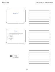
alternative sequences of instructions accordingly. The general form of the if statement is:
if logical expression
first group of statements
else
second group of statements
always
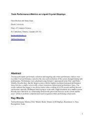
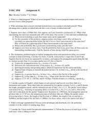
and may be flowcharted as shown in figure 1-1. In this figure, the first group of statements is executed
when the logical expression is true, and the second group of statements is executed when the
'logical expression' is false. The term "flow of control" is used to denote the sequence of instructions
followed under specific conditions, chosen from among the possible such sequences. The
keywords else and always may be replaced by alternative synonyms to improve the readability
of the if statement:
Else may also be expressed as otherwise
Always may also be expressed as regardless or endif
An example of the if statement is:
12

SIMSCRIPT II.5 Basic Concepts
if STATUS = BUSY
add 1 to NO.IN.QUEUE
else
let STATUS = BUSY
always
Here, a STATUS variable is tested against a value denoting BUSY status. The variable NO.IN.QUEUE
is incremented if the status flag is busy and the flow of control passes to always. Otherwise, the
status flag is set to reflect the now BUSY status and control naturally passes to the always statement.
logical
expression
False
ELSE
True
first group
of
statements
second group
of statements
ALWAYS
Figure 1-1. Flow of Control After an if Statement
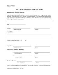
The else statement and 'second group of statements' are optional. There are cases when the choice
is simply whether or not to perform an action. This shortened form of the if statement is:
if logical expression
group of statements
always
13

SIMSCRIPT II.5 Programming Language
and is flowcharted in figure 1-2. When the logical expression is true, the group of statements is executed
and flow of control continues through the always statement. When the logical expression
is false, control transfers directly to the always. For example:
If X less than A
let A = X + Y
let B = X - Y
always
logical
expression
True
group
of
statements
False
ALWAYS
Figure 1-2. Flow of Control After Shortened if Statement
To improve program readability, the logical expression appearing in an if statement may be optionally
followed by a comma. The word is may also be used before the "English" versions of the
relational operators in logical expressions. Examples are:
if STATUS is not equal to BUSY,
if X is less than A,
Also, because logical comparisons with the value zero occur frequently in programming, the words
zero, positive, and negative may be combined with the words is and is not, replacing
14

SIMSCRIPT II.5 Basic Concepts
both the conditional operator and the right hand arithmetic expression, to form more readable logical
expressions in these special cases. Examples are:
if X is zero equivalent to if X = 0
if X-Y is positive equivalent to if X-Y > 0
if Z is not negative equivalent to if Z >= 0
Zero, positive, and negative may be thought of as properties associated with an arithmetic
expression. SIMSCRIPT II.5 allows for the expression of a number of such logical tests against
predefined properties. These will be presented in later sections as the context demands.
If statements can be "nested" by putting if statements within the statement group of other if statements,
thus allowing complex conditions to be specified. The statement group in an if statement
can contain any number of statements. The only qualification on this group is that it must be selfcontained
with respect to other if statements appearing within it. Each if is matched by a corresponding
always, as left parentheses are matched with right parentheses in an expression. For example,
the following program segment might be used to classify persons by age into one of the
groups CHILD, TEEN, or ADULT defined by the the age groups under 11 years, between 12 and 17
years, and over 18 years:
if AGE less than 12
add 1 to CHILD.COUNT
else
if AGE less than 18
add 1 to TEEN.COUNT
else
add 1 to ADULT.COUNT
always
always
To indicate program structure and flow of control, it is helpful to indent and align each if in a column
with its corresponding else, always, otherwise, regardless, or endif. Obviously,
an out-of-place else or always in a program can greatly alter the flow of control and thereby
the meaning.
A feature of one particular construct of nested if statements is that a failure to satisfy any one of
the logical conditions specified by any of the nested if statements effectively causes a transfer of
control out of the range of the entire nest. Such a structure is illustrated below:
if VALUE > 1000.00
let PRIORITY = 2
if TIME.DUE < 3
add 1 to PRIORITY
if WORKTIME < 1
add 1 to PRIORITY
always
always
always
15

SIMSCRIPT II.5 Programming Language
The failure of any test causes a transfer to one of the cascaded always statements, and hence a
transfer out of the structure. Successive if statements add further logical tests to that of the first
if statement. This structure may be simplified for readability by prefixing the word then to the
second and subsequent if statements, and eliminating all but one of the consecutive always statements.
The example shown above could be written as:
if VALUE > 100.00
let PRIORITY = 2
then if TIME.DUE < 3
add 1 to PRIORITY
then if WORKTIME < 1
add 1 to PRIORITY
always
Note that the then if construct is only applicable to nested logical tests in which the false condition
for any of the tests is to have the same effect — a transfer of control out of the nest structure.
While the use of then if may reduce the number of statements required, the programmer must
judge whether such use obscures the logical intent of the structure.
1.12 More on Logical Expressions
The logical expressions described above have used relational operators to specify comparison between
two arithmetic expressions, or between one such expression and defined properties such as
zero or negative. This section elaborates on the structure of logical expressions.
A logical expression may be negated by following it with the phrase is false, as in the expression:
value < LIMIT is false
The is false phrase may be used to improve readability by stating a desired condition without
forcing an unnatural transposition of logic. For example, a test may be written as:
or:
if QUANTITY > INVENTORY
let ORDER = ORDER - 1
always
if QUANTITY

SIMSCRIPT II.5 Basic Concepts
and or. (In this context, a comma cannot be substituted for the word.) If E1 and E2 are logical
expressions, then:
E1 and E2 is true if both E1 and E2 are true
E1 or E2 is true if either or both of E1 and E2 are true
Compound logical expressions may contain more than two simple logical expressions, as in the logical
expression:
E1 and E2 or E3 and E4
When more than two simple logical expressions appear in an unparenthesized compound logical expression
with the operators and or or, the operator and is evaluated first. Parentheses can be used,
however, to indicate a specific order of evaluation. In the absence of parentheses, the above expression
is, by convention, evaluated, as though it had been written:
(1) (E1 and E2) or (E3 and E4)
If a program requires some other logic, the statement can be written as:
(2) E1 and (E2 or E3) and E4
which means something quite different. Version (1) is true either if both E1 and E2 are true or if
both E3 and E4 are true. Version (2) is true if E1 is true and E4 is true, and either E2 or E3 is true.
Compound logical expressions can be used with is false and is true phrases. An is false
or is true phrase always applies to the logical expression preceding it. If this logical expression
is compound, it must be enclosed in parentheses, as shown in the logical expression:
E1 is false and (E2 or E3) is true
A few simple rules that govern the writing and evaluation of logical expressions are given below.
1. A logical expression enclosed in parentheses remains a logical expression.
2. In the absence of parentheses, and is evaluated before or. Successive logical expressions
are used as operands of and operators, and these evaluated expressions are then used as operands
of or operators. Parentheses can always be used to indicate specific operator hierarchies.
3. Is true and is false phrases apply to logical expressions preceding them. If such a
logical expression is compound, it must be enclosed in parentheses. Otherwise, the phrase
only applies to the expression adjacent to it.
Some examples that illustrate the writing and evaluation of complex logical expressions are given
below. In these examples, the variables I, J, K, M, and N are positive numbers; the variables Q,
R, S, and T are negative numbers; and the variable Z is zero.
17

SIMSCRIPT II.5 Programming Language
1. I equals J is true or false depending on the values I, J
2. I equals Q is always false
3. M + N is positive is always true
4. M + T is positive is true or false depending on the values M, T
5. I > 0 and J > 0 is always true
6. I > 0 or R > 0 is always true
7. I eq J and Z eq 0 is true if I equals J, and false otherwise
8. I eq J or Z eq 0 is always true
9. I = J and K > N and R = S is true if all three conditions are true, and
false otherwise; it is evaluated as ((I =
J) and (K > N) and (R = S))
10. I = J or K > N or R = S is true if any one of the three conditions
is true; it is false only if all are false
11. I = J and K > N or R = S is true if either of the two conditions
12. Z is zero and (I < 0 or S < 0) and Q = T is true if Q = T
13. Z is zero and (I > 0 or S < 0) and Q = T is true if Q = T
around the or is true; it is evaluated as
(I = J and K > N) or (R = S)
14. J< K and (I = Q or S < 0) and J + K < I is true if J < K and J + K < I
When a statement containing a compound logical expression is executed, it does not always follow
that all logical conditions in the statement are examined. For example, in the segment:
if X > Y**2 and COUNT > N
add ...
always
both logical expressions have to be true for the add statement to be executed. If the first logical
expression (X > Y**2) is false, there is no need to evaluate the second (COUNT > N), as the compound
logical expression X > Y**2 and COUNT > N can never be true regardless of the values of COUNT
and N. In normal circumstances, the fact that all the parts of a compound logical expression may
not be evaluated each time will cause no difficulty.
It should be noted that compound logical expressions formed using the logical operator and may
be written in an alternative way. Using e to represent an arithmetic expression and R to represent a
relational operator, such compound logical expressions may be written as:
Form
e R e
e R e R e
Example
1 < X
1 < X < N
18

SIMSCRIPT II.5 Basic Concepts
e R e R e R e
1 < X < N = SUM
e R e R e R e R e 1 < X < N = SUM is greater than 5
In each of these cases, all of the expressed logical relationships must be true in order for the compound
expression to be true. For example, in the second illustration, X must be greater than 1 and
less than N. Thus, the expression 1 < X < N is equivalent to 1 < X and X < N.
1.13 Repetition Using Control Phrases
Another important concept is that of repetition. Much of the power of the computer lies within its
ability to repeat a sequence of instructions. A SIMSCRIPT II.5 statement can be executed more
than once by prefixing it with a control phrase. An example of a control phrase prefixed to a statement
is:
for I = 1 to 3 by 1
print 1 line with I and I ** 2 thus
THE SQUARE OF * IS *
The control phrase, for I = 1 to 3 by 1, controls the execution of the print statement to
which it is prefixed, causing this statement to be repeated three times, first with I = 1, next with
I = 2, then with I = 3. To demonstrate, the example uses the value of the variable I within the
print statement, displaying the lines:
THE SQUARE OF 1 IS 1
THE SQUARE OF 2 IS 4
THE SQUARE OF 3 IS 9
The general form of a control phrase is:
for V = E1 to E2 by E3
where E1, E2, and E3 are arithmetic expressions, and V is a variable. E3 must be greater than
zero, or an error results.
The first time the control phrase prefixed to a statement is executed the control phrase variable V is
set equal to the value of E1. If the value of E1 is not greater than that of E2, the controlled statement
is executed. After execution, the value of E3 is added to the control phrase variable, and if this new
value is again less than E2, the controlled statement is repeated. This process continues, with the
control phrase variable taking on successively larger values until it exceeds the value of E2.
If the phrase by E3 is omitted from the control phrase, a value of 1.0 is assumed for E3. This form
is convenient when the control phrase is used simply to count the number of times a statement is
executed. A comma at the end of a control phrase is optional.
The following examples illustrate some control phrases and the successive values of their corresponding
control phrase variable:
19

SIMSCRIPT II.5 Programming Language
Examples of
Control Phrases
Successive Values of v
for I = 1 to 5, 1,2,3,4,5
for I = -5 to 5, -5,-4,-3,-2,-1,0,1,2,3,4,5,
for I = 0.0 to 2.0 by 0.5 0.0,0.5,1.0,1.5,2.0
for I = 10 to N by M,
If N is less than 10, the controlled statement will not
be executed.
If N is at least equal to 10, the controlled statement
will be executed with I=10, 10+M, 10+2*M, ...,
10+n*M until I exceeds N.
As stated earlier, the value of the expression E3 is added to the control phrase variable each time
the statement is repeated. A variant of the control phrase format causes the value of E3 to be subtracted,
and thus allows the control phrase variable to step backward:
for V back from E1 to E2 by E3
Everything applicable to the forward stepping control phrase applies to this phrase. The only difference
is in the direction in which the control phrase variable changes value. Again, E3 must be
greater than zero.
Control phrases can be nested together, providing more complex control over the repetition of statements:
for NUM = 1 to 12,
for MULT = 1 to 10,
print 1 line with MULT, NUM, and MULT * NUM thus
** TIMES ** IS ***
This example computes and prints the multiplication tables for each of the numbers from 1 to 12
and for multipliers from 1 to 10. Both control variables are used within the controlled statement,
producing the displayed result:
1 TIMES 1 IS 1
2 TIMES 1 IS 2
3 TIMES 1 IS 3
.
.
10 TIMES 1 IS 10
1 TIMES 2 IS 2
2 TIMES 2 IS 4
3 TIMES 2 IS 6
.
.
10 TIMES 12 IS 120
20

SIMSCRIPT II.5 Basic Concepts
Used in this way, the first control phrase is said to be an outer phrase, and the second phrase an inner
phrase. The controlled statement is repeated so that the inner phrase steps through the entire range
of values for the inner control phrase variable MULT for each new value of the outer control phrase
variable NUM.
An indefinite number of phrases can be nested together in this way. Each successive phrase is an
outer phrase of the following phrase and an inner phrase of the preceding phrase. Control variables
of outer phrases can be used in the expressions E1, E2, and E3 of inner phrases, as their values are
defined within these phrases. This usage will be explored in more detail in Chapter 2.
1.14 Control Phrases Extended To Cover More Than One Statement
The concept of a control phrase can be expanded to permit the phrase to control an arbitrary number
of statements. Statements to be controlled as a group are enclosed between the words do and loop.
A control phrase controls grouped statements in exactly the same way it controls a single statement.
As an example, consider a program, similar to the very first example, but extended to calculate the
sum of any 10 numbers supplied as input data. The variable TOTAL can be assumed to be initialized
to zero. However, it is explicitly assigned a zero value here to clarify the steps in this computation:
let TOTAL = 0
for COUNT = 1 to 10 by 1
do
read NUMBER
add NUMBER to TOTAL
loop
print 1 line with TOTAL as follows
THE SUM IS : ****
stop
The two grouped statements read a new value from the input data, assign its value to the variable
NUMBER, and then add this value to TOTAL. This group executes 10 times, after which the incremented
value of the control phrase variable, COUNT, halts the repetition. The flow of control passes to
the following statement that displays the result. Note that in this example COUNT is not used anywhere
within the controlled statements, but only to control the number of times the statements are
repeated.
A do loop (as we shall call this expanded structure hereafter) can also be constructed from a backward
iterating for phrase. Thus, we can write:
for I back from 10 to 1
do
.
.
loop
21

SIMSCRIPT II.5 Programming Language
It is common to indent in some regular way the statements that are to be repeated within the control
structure of a do loop (as for the statement groups in an if statement) drawing attention to the departure
from normal sequential flow of control.
The following program uses a number of terms from an infinite series to estimate an approximate
value for the irrational number PI. The value of PI, approximately 3.14159..., can be represented
by the infinite series:
PI/4 = 1 - 1/3 + 1/5 - 1/7 + 1/9 ...
The accuracy of the approximation is controlled by a variable read from input data. This data value
sets a limiting value on the size of the divisor in the terms of the series. The summation is halted
when the values of subsequent terms become too small to affect the desired accuracy of the result.
For example:
read LIMIT
let VALUE = 0
let SIGN = +1
for DIVISOR = 1 to LIMIT by 2
do
add SIGN/DIVISOR to VALUE
let SIGN = -SIGN
loop
print 1 line with VALUE*4 as
The Approximate Value of Pi is *.******
stop
The variable DIVISOR takes the values 1,3,5,... until it exceeds the limiting value. Note the
use of the unary operators to control the sign of successive terms.
1.15 Logical Control Phrases
Normally, a do loop, controlled by a for statement, is executed over the entire range of values of
the control variable generated. An alternative is to control the repetition of statements using some
logical condition that may be evaluated during the execution of the controlled statements.
A logical control phrase contains a logical control operator and a logical expression and may be
used to control a do loop. The logical control phrases are:
while logical expression
and
until logical expression
The following example illustrates the use of a logical control phrase in a program:
22

SIMSCRIPT II.5 Basic Concepts
while TOTAL.WEIGHT < LIMIT
do
read PASSENGER.NO, FARE, and BAGGAGE.WEIGHT
add BAGGAGE.WEIGHT to TOTAL.WEIGHT
add FARE to TOTAL.REVENUE
loop
In this example, the value of the variable TOTAL.WEIGHT is incremented for each set of passenger
data read. As long as TOTAL.WEIGHT does not equal or exceed the value LIMIT, the statements in
the do loop are repeated. When the logical condition becomes untrue, that is, TOTAL.WEIGHT
equals or exceeds LIMIT, the repetition terminates and control transfers to the statement following
loop.
An until phrase is similar to a while phrase, but the terminating condition may be expressed as
the logical complement of that used in the while phrase. The phrase:
until TOTAL.WEIGHT >= LIMIT
could be substituted for the while phrase in the above example with an identical effect. In the example
in the previous section, the calculation of an approximate value for PI, the accuracy of the
computation was controlled by an input data value limiting the magnitude of the divisor in included
terms of the series. It might seem more straightforward to specify directly a lower bound on the
size of the terms to be included in the summation. The following example uses an until phrase to
control the do loop:
read LOW.BOUND
let VALUE = 0
let SIGN = +1
let TERM = 1
let DIVISOR = +1
until TERM less than LOW.BOUND
do
add (TERM * SIGN) to VALUE
let DIVISOR = DIVISOR + 2
let SIGN = -SIGN
let TERM = 1/DIVISOR
loop
print 1 line with VALUE*4 as
The Approximate Value of Pi is *.******
stop
Recalling that for control phrases may control the repetition of single statements as well as do
loops, note that while and until statements may be used in the same way. Because a single statement
may not, for the present, appear to offer much scope for altering the logical condition, the usefulness
of this construction may not be immediately appreciated. It is mentioned here for
completeness and will be expanded on in later chapters.
23

SIMSCRIPT II.5 Programming Language
Because there is no automatic termination of a do loop controlled by a while or until phrase, as
there is with a for phrase, care must be taken not to program a nonterminating loop, as in the following
program segment:
while NUMBER.OF.SEATS is not zero
do
read PASSENGER.NO, FARE, and BAGGAGE.WEIGHT
add BAGGAGE.WEIGHT to TOTAL.WEIGHT
loop
This loop is not terminal, as the value of NUMBER.OF.SEATS is not affected by any statement within
the do loop, and hence, if the logical expression is true when the loop is initiated, the condition
will never become false. One means of avoiding this problem is to use a combination of a for control
phrase modified by a logical control phrase. A while phrase, for example, may be used to allow
a for phrase to direct the sequence of program control as long as a specified logical expression
is true. The logical expression is reevaluated each time the for phrase changes the value of its control
variable. Thus, the loop in the following example may be terminated either when all seats have
been allocated or when the total baggage weight exceeds the allowable limit:
for COUNT = 1 to NUMBER.OF.SEATS,
while TOTAL.WEIGHT not greater than LIMIT
do
read PASSENGER.NO, FARE, and BAGGAGE.WEIGHT
add BAGGAGE.WEIGHT to TOTAL.WEIGHT
loop
This example could have been written equally well using an until phrase:
for COUNT = 1 to NUMBER.OF.SEATS
until TOTAL.WEIGHT > LIMIT
do
.
.
Two additional logical control phrases, with a rather different effect, may be used to modify statement
repetition, as so far discussed. These are:
and
with logical expression
unless logical expression
Unlike while and until phrases that control the termination of repetition, a with phrase may be
used to selectively control whether or not the statements are executed at each repetition. For example,
a with phrase modifies the sequence of values that pass from a for phrase to the statements
that it controls. The logical expression is tested each time a new value of the for phrase control
variable is generated, and if the expression is false, then execution for this value of the control vari-
24

SIMSCRIPT II.5 Basic Concepts
able is skipped. This operation effectively passes control around the statements for a selected control
variable value or set of values. The phrase is useful for screening values before they pass into
for-phrase-controlled statements. A store, for example, that does business every weekday, except
Wednesday, might, in accounting for the weeks' sales, use the program statements:
for DAY = 1 to 6
with DAY not equal 3
do
read SALES.QUANTITY,...
.
.
loop
In this example, the with phrase causes the statements within the loop to be skipped for the value
3, which is generated as a value for DAY in the for sequence, and for which value the loop would
normally be executed.
The word when can be used as a synonym for with. The words unless or except when can
be used equivalently to show that the items passing the indicated test are screened from the loop,
rather than accepted. Hence, the above example could be written:
for DAY = 1 to 6
unless DAY = 3
do
.
.
With, unless, while, and until phrases can be attached to nested for statements. When this
is done, each with or unless phrase applies to the for statement immediately preceding it, and
each while or until phrase applies to all preceding for phrases. The example statement illustrates
this:
for DELTA = 1 to 100 by 0.5,
for Q = L1 to L2 by DELTA,
while (DELTA/Q) less than LIMIT
for V = -Q to Q by STEP,
with V ne 0
do
add ... to SUM
.
.
loop
The outer for phrases step the variables DELTA and Q through a sequence of values as long as the
logical expression in the while phrase is true. A false condition ends the for phrase control by
transferring to the next statement after the loop statement. Each time the variables are stepped and
the logical expression is true, the inner for steps the variable V through a sequence of values. Only
25

SIMSCRIPT II.5 Programming Language
those values in the sequence, however, for which the logical expression in the with phrase is true
(i.e., all values but zero) are passed on to the statements in the do loop.
Sequences of with, unless, while, and until phrases can be attached to for phrases in any
combination. More than one of each type of phrase is permitted. While and until control phrases
may also be modified by with and unless phrases, and may be nested with other independent
while and until phrases to control statement repetition. Again, the use of such combinations of
control phrases will become more apparent in later examples.
1.16 Altering the Flow of Control Within a Loop
There are occasions when it may be necessary to exercise more explicit direction on the flow of control
than may readily be specified using the control structures discussed so far. Consider the previous
example:
for COUNT = 1 to NUMBER.OF.SEATS,
while TOTAL.WEIGHT < LIMIT
do
read PASSENGER.NO, FARE, and BAGGAGE.WEIGHT
add BAGGAGE.WEIGHT to TOTAL.WEIGHT
loop
Examination of the statements within the loop shows that if the loop is terminated by the while
phrase, the weight of the last passenger's baggage must have overflowed the LIMIT value. This
may not be quite what was intended. The problem arises because the test of the condition is made
only at the beginning of the loop, and all the statements in the loop are executed at each iteration.
There are occasions when the test should logically be made within the loop. The following example
uses a leave statement to transfer control out of the loop when the LIMIT is about to be exceeded:
for COUNT = 1 to NUMBER.OF.SEATS
do
read PASSENGER.NO, FARE, and BAGGAGE.WEIGHT
if TOTAL.WEIGHT + BAGGAGE.WEIGHT > LIMIT
leave
otherwise
add BAGGAGE.WEIGHT to TOTAL.WEIGHT
loop
let LOAD.FACTOR = (COUNT-1)/NUMBER.OF.SEATS
.
.
The leave statement, which may only be used within a do loop, causes the flow of control to pass
to the statement immediately following the loop statement that delimits the do loop. This addition
to the construction of a do loop proves useful in those cases where the terminating condition is dependent
on some of the actions performed within the loop. Note the use of otherwise in this example.
This usage is discussed in the next paragraph. Note also that the value of the control phrase
26

SIMSCRIPT II.5 Basic Concepts
variable COUNT remains set to the value assigned at the last evaluation of the control phrase, and
may be used in subsequent computation.
The cycle statement bypasses any further statements within the do loop, beginning the evaluation
of the control phrases determining the next repetition. Again, this statement can be useful where
the tested condition is dependent on some evaluation made within the loop. Although one or more
if statements could be used to achieve a similar effect, the cycle statement makes it clear that
there is to be no further computation within this iteration of the loop.
for COUNT = 1 to NUMBER.OF.SEATS
do
read PASSENGER.NO, FARE, and BAGGAGE.WEIGHT
add BAGGAGE.WEIGHT to TOTAL.WEIGHT
if FARE is not equal to FIRST.CLASS.FARE
cycle
otherwise
read MENU.CHOICE, SEAT.SELECTION
if MENU.CHOICE = VEGETARIAN
.
.
always
loop
1.17 Changing the Flow of Control By Direct Order
The leave and cycle statements are two special cases of a generalized capability to directly control
the order in which statements are executed. Any statement in a program may be prefixed with
a label. A label is a name enclosed in single quotation marks (apostrophes). The flow of control
may then be directed to continue from this statement by executing a go to statement referencing
the label. The go to statement is of the form:
Go to 'label'
or
Go to label
The quotation marks are mandatory when the label is defined (i.e., when it appears in front of a referenced
statement), but optional when the label is referenced in a go to statement. The word to
is also optional. In Program 1-1, go to is used both to transfer out of the loop control if an error
condition is detected, and to transfer to a group of common statements after performing selective
processing for individual cases.
Note that the second group of statements and the terminating always is omitted when the first
statement group of an if group ends with an unconditional transfer of control (i.e., leave, cycle,
go to). In other words, an else or otherwise immediately preceded by go to is equivalent to
an always statement.
27

SIMSCRIPT II.5 Programming Language
Program 1-1.
_______________________________________________________________________________
for COUNT = 1 to NUMBER.OF.SEATS
do
read PASSENGER.NO, FARE, and BAGGAGE.WEIGHT
let CHECK.SUM = ...
if CHECK.SUM CHECK.VALUE
go to 'CHECK.ERROR'
otherwise
if FARE = FIRST.CLASS.FARE
add 1 to CHAMPAGNE.COUNT
go to 'TOTALS'
otherwise
if FARE = EXECUTIVE.CLASS.FARE
.
.
go to 'TOTALS'
otherwise
if FARE = ECONOMY.CLASS.FARE
.
.
go to 'TOTALS'
otherwise
if FARE = STANDBY.FARE
.
.
go to 'TOTALS'
otherwise
'TOTALS'
add BAGGAGE.WEIGHT to TOTAL.WEIGHT
add 1 to MEALS.REQUIRED
loop
let LOAD.FACTOR = (COUNT-1)/NUMBER.OF.SEATS
.
.
'CHECK.ERROR'
print 1 line with PASSENGER.NO thus
ERROR IN TICKET NO. ******
_______________________________________________________________________________
The otherwise (or the synonym else) in this example could be replaced by always, endif
or regardless with exactly the same meaning. This structure has been retained to provide
compatibility with earlier versions of the SIMSCRIPT language. To clearly identify this anomaly
in control structure, it is suggested that the otherwise synonym for else be reserved for this
usage.
28

SIMSCRIPT II.5 Basic Concepts
The go to statement provides great flexibility in directing the flow of control. However, it can
detract from the clarity of the logic and the readability of the program. Unwisely used, it can multiply
the possible paths through the program, rendering comprehension and testing of the logic unnecessarily
difficult. Structured programming principles suggest that the logic of a program should
be expressed in restricted control flow structures. In particular, the concepts of conditional action
and iteration should be represented using the if and do loop structures.
1.18 The Logical End of a Program
The stop statement is used to terminate a program. Because there may be more than one stop
statement in a program, and control flow may be diverted around any stop statement, it does not
always appear as the last statement of a program listing. The following program segment illustrates
the use of the stop statement in conjunction with an if statement:
if X is zero
print 1 line as follows
ZERO IS AN ILLEGAL VALUE FOR X
stop
otherwise
let Z = Y/X
Note: The stop statement is considered to be an unconditional transfer of control.
1.19 The Physical End of a Program
The last statement in every SIMSCRIPT II.5 program must be end. It signals that the entire source
program has been read. The example programs at the end of this chapter illustrate the use of the
end statement.
1.20 A Note on SIMSCRIPT II.5 Program Form
SIMSCRIPT II.5 programs are composed of sequences of conventionally arranged symbols —
some are standardized key words such as let and read and others are programmer-constructed
variable names and numeric constants. The basic symbolic units recognized by the SIMSCRIPT
II.5 compiler in scanning program statements are names and numbers, the special characters +, -, ',
*, /, **, (, ), ", >,

SIMSCRIPT II.5 Programming Language
key words) in statements. Two adjacent statement words must always be separated by at least one
blank unless one of them is a special character. Thus:
let X = Y
can be written as:
let X=Y
but not:
letX=Y,
and:
if (SIGN + 5) is greater than DELTA
can be written as:
if(SIGN+5) is greater than DELTA
but not as:
if(SIGN+5) isgreaterthanDELTA.
Merely looking at a statement usually makes it clear whether a blank is needed or not. Because multiple
blanks are treated as single blanks, blank characters can be freely used to improve the readability
of statements, as many of the illustrations in this book demonstrate.
Statements can be typed as desired in a program, with one slight restriction. A statement can be written
on more than one input line, or several statements can be written on the same line, but statement
words (names, numbers, and key words) cannot be split between lines. Consequently, names and
constants are restricted to the length of one record. (Remember that the exponentiation symbol **
is a single unit and cannot be split.) Statement labels, where used, must precede the statement but
need not appear on the same line as the statement. More than one label may be prefixed to a single
statement.
The logical structure of a program should be reflected in the physical layout. The use of indenting
to draw attention to a departure from sequential execution of statements is one example. The use
of appropriate control structures, rather than ad hoc direction of control flow through go to, can
contribute greatly to this goal.
1.21 Clarifying Comments In a Program
Whenever it appears that a clarifying remark would be helpful to the reader, a comment should be
used. A comment is delimited on the left by two single apostrophes (''). Comments can appear
anywhere in a program except within a word. They may appear on the same line as program statements
or on separate lines. Comments serve only as documentation, but they should be used wher-
30

SIMSCRIPT II.5 Basic Concepts
ever the logical intent of a program is not immediately evident from its SIMSCRIPT II.5 instruction
sequences. The use of comments will be illustrated in many of the example programs below.
1.22 Some Sample SIMSCRIPT II.5 Level 1 Programs
The following programs illustrate the SIMSCRIPT II.5 concepts and statements presented in this
chapter. The programs are printed as they might appear before being submitted for compilation.
The flexibility of SIMSCRIPT II.5 makes many program statement formats possible. Those used
here are examples only.
1.22.1 Roots of a Quadratic Expression
The following example, demonstrating the use of nested if statements, calculates the roots of a
quadratic equation, which may be expressed in the general form:
AX 2 + BX + C = 0
First, the coefficients, A, B, and C, are read from input data. They are printed so that they may be
checked for any input errors. The coefficients are then tested for the trivial zero, constant, or linear
cases. Otherwise, the roots, alpha and beta, may be calculated from the familiar formulae:
alpha = -B + (B**2 - 4AC)**(1/2)
2A
beta = -B - (B**2 - 4AC)**(1/2)
2A
Before obtaining the square root, the sign of the sub-expression B 2 - 4AC is evaluated. If this value
is less than zero, the roots have complex values; otherwise, real values. Notice how the print
statement, as used in the example, can be used to print both the program title and the labeled variable
names.
31

SIMSCRIPT II.5 Programming Language
Program 1-2.
_______________________________________________________________________________
'' Program To Compute The Roots of a Quadratic Equation
'' of the Form AX**2 + BX + C = 0
read A,B,C
print 2 lines with A,B,C as follows
ROOTS OF THE QUADRATIC EQUATION WITH COEFFICIENTS:
A=***.** B=***.** C=***.**
if A eq 0
if B eq 0
if C eq 0
print 1 line as follows
TRIVIAL CASE, COEFFICIENTS ALL ZERO
else
print 1 line with C as follows
EQUATION STATES ***.** = 0
always
else
print 1 line with -C/B as follows
LINEAR, ONE ROOT ALPHA = ***.**
always
else
let X = B**2 - 4*A*C
if X ls 0
let IMAG = ( (-X)**0.5 )/(2*A)
let REAL = -B/(2*A)
print 2 lines with REAL,IMAG as follows
EQUATION HAS COMPLEX ROOTS
REAL PART = ***.** IMAGINARY PART = ***.**
else
let X = X ** 0.5
let ALPHA = (-B+X)/(2*A)
let BETA = (-B-X)/(2*A)
print 2 lines with ALPHA,BETA as follows
EQUATION HAS REAL ROOTS
ALPHA = ***.** BETA = ***.**
always
always
stop
end
_______________________________________________________________________________
1.22.2 Finding the Area of a Triangle
This program demonstrates nested if statements, using more complex logical expressions. The
program calculates the area and perimeter of a triangle with the lengths of the sides A, B, and C as
input data. The first if statement verifies that none of the sides is of zero or negative length. The
32

SIMSCRIPT II.5 Basic Concepts
second if statement checks that the values read will form a triangle, based on the condition that the
sum of the lengths of any two sides is greater than the length of the remaining side. All three conditions
of the if statement must prove false before control is passed to the group of statements that
calculates the area and perimeter.
Program 1-3.
_______________________________________________________________________________
‘’Program to Compute the Area and Perimeter of a Triangle
‘’Given the Lengths of the Sides
read A,B,C
print 2 lines with A,B,C as follows
CALCULATE AREA OF A TRIANGLE WITH FOLLOWING SIDES:
A=**.** B=**.** C=**.**
if A

SIMSCRIPT II.5 Programming Language
Program 1-4.
_______________________________________________________________________________
''Program to Compute the Maximum, Minimum and Average
'' of a Set of Numbers
read NUMBER
'' NUMBER OF DATA OBSERVATIONS
if NUMBER < 1
go to FINISH
otherwise
read VALUE
let MAX = VALUE
let MIN = VALUE
let SUM = VALUE
for COUNT = 2 to NUMBER by 1
do
read VALUE '' DATA VALUE
add VALUE to SUM
if VALUE > MAX
let MAX = VALUE
always
if VALUE < MIN
let MIN = VALUE
always
loop
print 3 lines with SUM / NUMBER, MAX, MIN thus
THE AVERAGE VALUE IS ***.****
THE MAXIMUM VALUE IS ***.****
THE MINIMUM VALUE IS ***.****
'FINISH'
stop
end
_______________________________________________________________________________
1.22.4 Computing Square Roots
The square root of a number is required in many calculations. In fact, in two of the preceding examples,
square roots were obtained using exponentiation. The following is an implementation of
Newton's method to approximate square roots.
The example demonstrates the use of a logical control phrase to control an iterative computation.
The logical condition specifies a relative precision of the estimated square root as a stopping
criterion. Note that the first statement within the loop calculates a new estimate for the square root,
using the last estimated value. This technique is fundamental to such iterative procedures. Note
also the explanatory comment appearing beside the statement to invert the sign of DELTA, should it
be negative.
34

SIMSCRIPT II.5 Basic Concepts
Program 1-5.
_______________________________________________________________________________
''Program to Calculate Approximate Square Roots
read NUMBER
if NUMBER is not positive
print 1 line thus
CANNOT EVALUATE SQUARE ROOT: VALUE NOT POSITIVE
else
let SQRT = NUMBER/2.0
let DELTA = SQRT
until DELTA < (0.00001 * SQRT)
do
let SQRT = (SQRT + NUMBER/SQRT)/2.0
let DELTA = NUMBER/SQRT - SQRT
if DELTA is not positive
let DELTA = -DELTA '' USE THE ABSOLUTE VALUE
always
loop
print 1 line with NUMBER, SQRT thus
THE SQUARE ROOT OF *******.**** IS ****.*****
always
stop
end
_______________________________________________________________________________
35

SIMSCRIPT II.5 Programming Language
36

2. Programming Language Concepts
2.1 Variable and Label Names Revisited
Chapter 1 defined variable and label names separately. A variable name is any combination of letters
and digits that contains at least one letter. A label is any combination of letters and digits without
the "at least one letter" constraint. These rules can be expanded easily to permit more readable
programs by incorporating periods into the definition of names and labels.
Let a name be any combination of letters, digits, and periods that contains at least one letter or two
or more nonterminal periods. A constant is any combination of digits, possibly containing one period.
A variable name must look like a name and a label can look like a name or a constant. Thus,
variables can be distinguished from numbers while maintaining the widest latitude in name formation.
Some examples of variable and label names are shown in table 2-1.
Table 2-1. Variable and Label Names
_______________________________________________________________________________
Variable Names
PART.NUMBER
NUMBER.OF.PARTS
TOTAL
Label Names
LABEL
SECTION.1
PART.4
.PAGE
ERROR
_______________________________________________________________________________
As mentioned previously, it must be stressed that terminal periods cannot be used in distinguishing
names. The names X, X..., and X... all represent the same variable value; the labels '5' and '5.'
are identical.
Although SIMSCRIPT II.5 does not prohibit the use of any particular words (the one exception is
the word and, which should not be used as a name) or names, there are a number of special names
that are recognized in certain contexts. Guard against using any of these names incorrectly by
remembering the special naming conventions used for them. Some of these names are listed in
Appendix B, under various headings. Each of these names either begins with a letter followed by
a period or ends with a period followed by a letter, so it is good practice to not name your own
variables the same way!
2.2 Variable Modes
In the previous discussion, it was assumed that variables in SIMSCRIPT II.5 take on numeric values.
No explicit restrictions have been placed on the magnitude or precision of the numbers represented
by variable names. Complete freedom from concern over the expression of numeric
37

SIMSCRIPT II.5 Programming Language
quantities is an attractive idea. However, both the range and number of real numbers are infinite,
while a computer has a finite range of representations.
The enumeration of items, or iterations, requires the exact representation of a sizable range of integer
numbers. Many other calculations require the representation of a potentially greater range in
magnitude of the real numbers but are necessarily limited in accuracy.
Most computer systems, therefore, provide two internal representations for numeric data — one
trading some exactness of representation for increased range. These representations may vary between
different computer systems. The precise limitations pertaining to any SIMSCRIPT II.5 implementation
may be found in the appropriate user's guide. A programming language is used to
describe both the actions and the data on which these actions are to be performed. In this chapter,
some of the ways in which data are described are discussed.
A variable definition statement serves to declare the properties of a variable. This information is
used to determine the way in which the variable may be manipulated.
2.2.1 REAL and INTEGER Variables
SIMSCRIPT II.5 numeric variables may be declared to be integer or real. Variables declared
as integer represent only whole numbers. Variables declared as real represent numbers that can
have fractional values. Note that a whole number, lying within an established range of the integer
values, may be represented either by an integer or real variable. It is the possibility of a fractional
value, and not any particular value, that makes a variable require a real definition. The
numbers 56, -6745, 91, -1, and 0 are integer-valued. The numbers 56.0, 35.7846, 0.999876, -
27.45, and 0.0. are real-valued.
Every SIMSCRIPT II.5 program has a preamble that contains variable definition information. In
some cases, as in the previous examples, this preamble is implied but need not be written as all
variables are treated as real. Whenever a variable has a property that differs from one that
SIMSCRIPT II.5 assumes, a variable definition statement must be used. Programs containing an
explicit preamble begin with the one-word statement preamble. This section, containing variable
definition statements, is separated from succeeding program action statements by the word end.
As stated, the mode of a numeric variable is assumed real unless otherwise specified. The "normal
form" of SIMSCRIPT II.5 variables is real numbers. The assumed real condition can be changed
by using the statement:
mode is integer
This statement resets the compiler's "background conditions" so that all following program variables
are assumed integer unless otherwise specified. Mode is but one of several properties that
can be used to describe variables. Hence, the general form of the normally statement is:
normally, specification phrase list
38

Programming Language Concepts
Specification phrases may appear in the list in any order, separated, as usual, by commas or and.
The comma after the word normally is optional. The equals symbol (=) may replace the word is.
As additional specification phrases are added in later sections, phrase choices will be increased but
these rules will not change.
Another possibility is to force explicit definition of all variables by use of the form:
normally, mode is undefined
This will produce a diagnostic for every undefined variable. This form is strongly recommended in
order to guard against inadvertent background definition of misspelled variables.
Individual variables that differ from the implied or normally defined mode can have their mode
specified in a define statement. This statement lists one or more variable names and defines their
common mode. The statement:
define X, Y, Z as integer variables
illustrates the way in which the define statement is used to declare that the variables X, Y, Z
represent only integer values. If the background conditions were declared to be integer, a similar
define statement using the word real might be used to define some variables as real.
The define statement has a number of alternative forms. The only words that must appear are
define, the variable names being defined, as, and the word variable or variables. The words
a, an, integer, and real are included when needed. Some examples of the define statement
are:
define X as a real variable
define X and Y as integer variables
define X, Y, Z as variables
define X as a variable
The description of the define statement, like the normally statement, will be expanded in later
paragraphs to include more than variable mode definition.
Some computer systems provide an internal numeric representation of real numbers with an
increased precision, usually achieved by doubling the size of the internal binary representation.
SIMSCRIPT II.5 allows variables to be declared with this representation, by the use of the variable
mode double. On these systems, the normal background condition is double to allow the
maximum precision for decimal values. The appropriate SIMSCRIPT II.5 user's manual should be
consulted to determine whether this variable mode is implemented. In general, on those systems
that do not support this mode, double is interpreted as real.
Throughout this book, the behavior ascribed to real variables may be assumed to extend to
double variables. Examples of declarations are:
define AMOUNT, INTEREST as double variables
39

SIMSCRIPT II.5 Programming Language
and
normally, mode is double
2.3 Expression Modes
Although statements that combine integer and real variables are allowed, a programmer should
be aware of the way in which computations are carried out whenever using "mixed mode" expressions.
When A and B represent two variables, constants, or sub-expressions, then:
1. Arithmetic expressions of the form A op B, where A and B represent variables of specified
mode, or constants of that mode, and op is any of the arithmetic operations +, -, and *, are
integer if both A and B are integer, and real if either A or B is real.
2. Expressions of the form A/B are always real (Two integer expressions can be divided to
yield a truncated integer result by a library function called div.f. Library functions are
described in paragraph 2.15).
3. Expressions of the form A**B are always real.
Compound expressions are evaluated from left to right as a sequence of simple expressions that are
evaluated according to the above rules. In the following examples, if A, B, and C are integer,
then:
A/B + C
A + B + C
A**B + C
is real
is integer
is real
When an expression appears on the right-hand side of a let statement or in an add or subtract
statement, and its mode differs from the mode of the variable on the left-hand side, the expression
is converted to the mode of the variable before the value of the variable is changed. When the arithmetic
expression constituents of logical expressions differ in mode, all integer expressions are
converted to real before evaluating the logical expression as true or false.
Conversions from integer to real are straightforward. An integer to real conversion takes
the whole number that is the value of an integer variable and converts it to a real number with
the same value; 25 becomes 25.0, -11 becomes -11.0, and so forth.
Real to integer conversions are more complex. Obviously, any fractional part cannot be represented
by the integer. Real values are rounded to whole numbers by adding +0.5 to the variable
if its value is positive or -0.5 if it is negative, and truncating the result. If X is integer and e is
some real-valued expression (formed according to the above rules), then:
let X = e sets X = 0 if e = 0.2 since 0.2 + 0.5 = 0.7 → 0
let X = e sets X = 1 if e = 1.4999 since 1.4999 + 0.5 = 1.9999 → 1
let X = e sets X = 2 if e = 1.50000 since 1.50000 + 0.5 = 2.0000 → 2
40

Programming Language Concepts
Where double variables are supported, conversions between double and integer modes follow
the same procedures as conversions between integer and real. Hence, expressions mixing
integer and double arithmetic operations follow the procedure outlined above for mixed
integer and real expressions.
Expressions containing mixed double and real variables are evaluated to yield a double precision
result, which may be automatically converted to the real mode, if necessary. When required
by context, as in mixed real and double mode expressions, real values are automatically converted
to double before evaluation.
If, in the following examples, R has been defined as a real variable and D as a double variable,
then in executing the statement:
let D = D + R
R is converted to double before the addition, which produces a double precision result, while:
let R = R * D
converts R to double before the multiplication, but the result is truncated to real before reassignment.
As may be seen, the provision of different modes of variable representation brings with it some additional
complexity. A variable defined with a certain mode can only be used in ways consistent
with its definition. In some cases, automatic conversion between modes is performed as indicated
above, although information may be lost as in the case of real to integer conversion, where the
fractional value may no longer be represented. Be aware of such implied conversions and their effect
on program behavior.
One particular potential source of error, however, is the attempted assignment of variable values
read from input data to variables defined with conflicting internal representation. Specifically, a
data field containing a noninteger format number should not be assigned to an integer variable
in a read statement. This will result in loss of information and is therefore treated as an error condition.
Table 2-2 specifies the actions taken when different combinations of data and variable definitions
occur.
41

SIMSCRIPT II.5 Programming Language
Table 2-2. Real-Integer Input Data Conversions
______________________________________________________________________________
Input Data
Variable
Format Defined as Action
integer integer Data value stored in variable
integer real Data value converted to decimal representation
and then stored in variable; e.g., 55
stored as 55.0
real real Data value stored in variable
real integer Program terminates with error message; not
possible to store fractional value in integer
representation.
_______________________________________________________________________________
2.4 System-Defined Constants
Scientific and engineering calculations often involve standard scientific constants. Mathematical
computations frequently require values of numeric constants. Numbers such as PI = 3.14159..., and
e = 2.718... are examples of well-known and often-used constants.SIMSCRIPT II.5 maintains a library
of standard values. When the name of a library constant is used in a SIMSCRIPT II.5 program,
the correct numeric value of the constant is inserted in its place. These constants may be used
wherever a numeric literal constant could be used.
Library constants have names that look like variable names except that they end in the characters
.c (a naming convention used by the SIMSCRIPT II.5 system). The library constants and their values
are listed in table 2-3.
42

Programming Language Concepts
Table 2-3. System-Defined Constants
______________________________________________________________________________
Standard
Name Symbol Value Units Mode
pi.c p 3.141159265 -- Real *
Exp.c e 2.718281828 -- Real *
inf.c ∞ Largest value -- Integer
computer can store
Rinf.c ∞ Largest value -- Real *
computer can store
Radian.c - 57.29577 Degrees/radian Real *
* On systems that support additional precision, these constants are of double mode.
_______________________________________________________________________________
2.5 Subscripted Variables
Variables as described above may represent single, numeric data items in SIMSCRIPT II.5. A feature
of many programming languages is the facility to represent and manipulate data in a way that
reflects the natural structure of the data. Data occurring in the form of lists or tables, for example,
have a regular structure. SIMSCRIPT II.5 provides a structure by which a number of similar data
items, the array elements, may be collectively referenced by a single name, while each individual
element may be referenced by subscripting the array name with an index value.
A simply ordered collection of data items, such as a list (figure 2-1), is represented by a one-dimensional
array. The elements of this array can be referenced by an identifying name, LIST, for example,
and an index number, called the array subscript, which can assume integer values from 1 up to
the total number of elements in the list. The array name is used to identify the collection of elements.
The subscript, enclosed in parentheses after the array name, is used to denote particular elements.
Thus, the name of the variable that is the first element in the array LIST is LIST(1), the
fifth element is called LIST(5), and the I th element is LIST(I). Figure 2-2 shows the list of figure
2-1 with the individual element names inserted.
Figure 2-1. A List Structure: One-dimensional Array
43

SIMSCRIPT II.5 Programming Language
LIST(1) LIST(2) LIST(3) LIST(4) LIST(5) LIST(6) LIST(7) LIST(8) LIST(9)
Figure 2-2. Elements of a One-dimentional Array Called LIST
To demonstrate the use of such a structure, consider the problem of determining the date as the day
of the month, given the day number within the year. Clearly, the number of days within each month
are 12 items of data that might be used in some orderly, repetitive computation. These values could
be represented as the elements of a one-dimensional integer array, DAYS, indexed by month.
Thus, DAYS(1) would have a value of 31, DAYS(2) a value of 28 (ignoring the complication of
leap years for the present), and so forth. The program segment:
read DAYNUM
for MONTH = 1 to 12 by 1
while DAYNUM gt DAYS(MONTH)
do
subtract DAYS(MONTH) from DAYNUM
loop
print 1 line with DAYNUM, MONTH thus...
The **th day of the **th month
successively subtracts the values of DAYS(1), DAYS(2), and so on from the input value, DAYNUM,
until it comes within the range of the number of days in some month. In this case, the use of the
array provides representation of the data in a way that matches the repetitive processing capability
of the do... loop.
The array elements need not, of course, be accessed in order. The array structure provides
immediate access to any individual element, selected by subscript. Consider a computer program
to maintain an inventory of goods. Each item in the inventory is allocated a code number. An
integer array, STOCK, holds in each element, indexed by the item code, account of the number of
such items currently in stock. This information might be updated, during the processing of an order,
by the program statements:
read ITEM.CODE and QUANTITY
subtract QUANTITY from STOCK(ITEM.CODE)
Although all elements of a one-dimensional array must be similar, these elements may themselves
be arrays. A table of data items (figure 2-3), for example, may be represented by a one-dimensional
array where each element represents a row of the table as a one-dimensional array of data items ordered
by column number. Such a structure is termed a two-dimensional array.
44

Programming Language Concepts
Column 1 Column 2 Column 3 Column 4 Column 5
Row 1
Row 2
Row 3
Figure 2-3. A Table Structure: A Two-dimensional Array
Variables with a two-dimensional array structure are referenced by an identifier and a pair of subscripts.
The first subscript identifies a selected one-dimensional array. The second identifies a particular
element within this array. Figure 2-4 shows the two-dimensional array of figure 2-3, here
called TABLE, with the individual element names inserted. Note how the subscript values indicate
each element's position in the structure of the table. The identifier (as before) is the name of the
complete array structure. The subscripts are enclosed in parentheses and separated by a comma.
Each subscript is associated with an element location in one coordinate dimension. In figure 2-4,
the first subscript is used as the element location in the row direction, and the second as the element
location in the column direction.
This data structuring is not limited to two dimensions. In general, a data collection that has n reference
indices can be represented as an n-dimensional array structure. A three-dimensional array
called CUBE might have elements CUBE(I,J,K). A seven-dimensional array called SEVEN.DIM
might have elements SEVEN.DIM(A,B,C,D,E,F,G).
Subscripted variables (the elements of arrays) share the same range of possible modes as unsubscripted
variables. All elements of any one array, however, must be of the same mode. If their
mode differs from that of the background conditions set within a program, it can be declared in a
define statement in the same way as with unsubscripted variables. For instance, if the assumed
mode of all as yet undeclared variables has been set to real, write the statement:
define LIST and TABLE as integer arrays
Column 1 Column 2 Column 3 Column 4 Column 5
Row 1 TABLE(1,1) TABLE(1,2) TABLE(1,3) TABLE(1,4) TABLE(1,5)
Row 2 TABLE(2,1) TABLE(2,2) TABLE(2,3) TABLE(2,4) TABLE(2,5)
Row 3 TABLE(3,1) TABLE(3,2) TABLE(3,3) TABLE(3,4) TABLE(3,5)
Figure 2-4. Elements of a Two-dimensional Array Called TABLE
The dimensionality of an array, whether it has 0, 1, 2, 3 or more subscripts, should also be declared
in the preamble. A dimensionality specification phrase can be included in either normally or
45

SIMSCRIPT II.5 Programming Language
define statements, depending on whether it is to apply as a background condition or to specifically
named arrays. The phrase is written somewhat differently in each case.
An n-dimensional array background condition may be declared with a normally statement using
the phrase:
dimension is n
as in the statements:
normally dimension is 1
normally, mode is integer, dimension is 2
In a define statement, a dimensionality specification can be made for a list of subscripted variables
with the dimensionality phrase n-dimensional as in the statements:
define LIST as an integer, 1-dimensional array
define LIST and VECTOR as real, 1-dimensional arrays
define CUBE as a 3-dimensional, integer array
In general, if a majority of program variables share some definable property, this may be declared
as a background condition, using a normally statement. Define statements may then be used to
override this specification for specific variables, as in the example:
preamble
normally, mode is integer, dimension is 2
define X, Y, Z and Q as real variables
define VECTOR as a 1-dimensional array
end
A variable must not, however, be used in more than one define statement. It is permissible to
write:
normally, mode is real, dimension is 1
define X as an integer, 0-dimensional variable
It is not permissible to write:
normally, mode is real, dimension is 1
define X as an integer variable
.
.
define X as a 0-dimensional variable
Each unsubscripted (zero-dimensional) variable requires a location in computer memory in which
to record its current value at any time. Similarly, each element of each array requires a distinct
memory location where its value can be stored. A one-dimensional array with 10 elements uses 10
such memory locations, a two-dimensional array with 3 rows and 5 columns uses (3*5) = 15 memory
locations, and so forth.
46

Programming Language Concepts
The allocation of space within computer memory to unsubscripted variables is done automatically.
This automatic allocation cannot be made for subscripted variables. An array may have any number
of elements, and space cannot be allocated until this number is known.
The reserve statement is used to explicitly allocate computer memory space for arrays. The dimensionality
of each array is indicated by asterisks in subscript positions. Subscript size expressions
declare the largest value that each subscript position index can assume. The maximum
subscript values may also be referred to as the array dimensions or bounds. The product of these
expressions is used to determine the total space requirement of the array. Thus, the statement:
reserve LIST(*) as 9
allocates memory space for the 9 elements, LIST(1),LIST(2),...,LIST(9) of the one-dimensional
array called LIST, and the statement:
reserve TABLE(*,*) as 3 by 5
allocates space for the elements of the two-dimensional array TABLE.
A reserve statement is an executable statement, rather than a declaration, and thus can not appear
in the preamble of a SIMSCRIPT II.5 program. Until a reserve statement for an array has been
executed, storage is not allocated for that array, and its element values are not defined. Each subscripted
variable must, therefore, be reserved before it can be used. Any attempt to reference a subscripted
variable before space for it has been allocated will cause an error in program execution.
All the element values of an array are initialized to zero at the time memory space is allocated.
If a reserve statement specifying an array to which space is already allocated is encountered, no
action is taken and no further space is allocated. Even if the second reserve statement specifies
a different size, the amount of space allocated is as given by the first reserve.
More than one array allocation may be made by a single reserve statement. The effect of the two
statements shown could be achieved by executing the statement:
reserve LIST(*) as 9, TABLE(*,*) as 3 by 5
If an array name appears in a reserve statement without asterisks to indicate its subscript positions,
the dimensionality previously declared in a define statement is understood. If no dimensionality
declaration has been made, the number of subscript size expressions is used to determine
the dimensionality. Thus, if an array has been declared as two-dimensional by the statement:
define MATRIX as a 2-dimensional, integer array
or, if no dimensionality declaration has been made for the array, the statement:
reserve MATRIX as 5 by 7
is understood to mean:
47

SIMSCRIPT II.5 Programming Language
reserve MATRIX(*,*) as 5 by 7
The dimensionality of an array, then, is frozen either by explicit declaration in a define statement,
or when it is first referenced in an executable statement — which, of course, should be a reserve
statement. Although the dimensionality of an array may be apparent from the context, the explicit
declaration is recommended as an aid to program documentation. Once the array dimensionality
has been frozen, the array must be referenced consistently. Any inconsistent reference is detected
as an error during program compilation.
Subscript size expressions may be arithmetic expressions containing variables, including other subscripted
variables. If such expressions are real, they are rounded to integer before they are used
as array dimension specifiers. Thus, the statement:
reserve LIST(*) as N, TABLE (*,*) as N by 2*M
allocates space for the arrays LIST and TABLE where the space requirement is dependent on the values
of the variables N and M.
A subscript size expression should not evaluate to zero or a negative value. An attempt to reserve
space using a zero- or negative-valued size expression will cause a program to terminate with an
error message. If any subscript expression in a reserve statement evaluates to 1, there is only one
element allocated to that dimension of the array. The statement:
reserve X(*) as 1, Y(*,*) as 1 by 3
allocates space to an array X with one element, X(1), and a two-dimensional array Y with three elements,
Y(1,1), Y(1,2), and Y(1,3). For all practical purposes, these one- and two-dimensional
arrays are equivalent to the unsubscripted variable X and a one-dimensional array Y.
When two or more arrays are to be allocated with the same dimensions, they may be combined in
a list of array names. Thus, the following is acceptable:
reserve A (*,*), B(*,*), C(*,*) as 5 by 10
Any reserve statement can contain a sublist of this form among its list of arrays, as in:
reserve VECTOR(*) as 5,
A(*), B(*) and C(*) as 15,
LIST1(*) and LIST2(*) as N+M,
TABLE(*,*) as 3 by Y,
.
.
48

Programming Language Concepts
2.6 Reading Subscripted Variables
Subscripted variable values can be assigned from input data by including each element of an array
in the variable name list of a read statement. In the following examples, let LIST be a singly subscripted
variable allocated by the statement reserve LIST(*) as 10.
Individual elements of the array are read by listing their names (the array identifier followed by the
appropriate subscript expression(s) enclosed in parentheses) in the list of a read statement. Values
of LIST(1), LIST(5), and LIST(9) are read by the statement:
read LIST(1), LIST(5), LIST(9)
A variable name list can contain array elements whose subscript designators are expressions, such
as LIST(N*M+2/J) or LIST(I), as long as the variables appearing in these expressions have had
values assigned to them. Note that, as the variables named in a read statement are processed from
left to right, variables to be used as subscripts may be assigned if they appear in a read statement
before their subsequent use in the same statement as subscripts, as in:
read N, M, LIST(N), LIST(LIST(N) + M)
This example shows that both unsubscripted and subscripted variables can appear in the same read
statement list.
This procedure is obviously tedious for large arrays, and so provision is also made for reading all
the values of a subscripted array, in order, by including the unsubscripted array name in the list.
Read LIST reads the 10 elements of LIST, as defined by the reserve statement. Numbers are
read and assigned to the elements of LIST in increasing subscript order: the first data item is
assigned to LIST(1), the next to LIST(2), and so on. If LIST were a multidimensional array, the
data would be assigned to successive elements whose subscripts change in increasing order, with
the last subscript position varying most rapidly. A two-dimensional array is read in row-by-row, as
in TABLE(1,1), TABLE(1,2), TABLE(1,3), ..., TABLE(1,N), TABLE (2,1),
TABLE(2,2), ..., TABLE(2,N), etc.
Mixtures of unsubscripted variables, elements of arrays, and entire arrays can be read in one read
statement. In the following example, if LIST and VECTOR are one-dimensional arrays and X and Y
unsubscripted variables, the statement:
read X, LIST(Y), VECTOR
reads a data item and assigns its value to X, reads another data item and assigns its value to
LIST(Y), and then reads as many values as there are elements reserved in VECTOR.
Clearly, the repetition provided by the use of a control phrase is useful when processing the elements
of subscripted variables. Such a control phrase may be used to govern the reading of array
values. The following statement reads N data values, assigning them to the first N elements of the
array LIST:
49

SIMSCRIPT II.5 Programming Language
for I = 1 to N
read LIST(I)
If N were the reserved dimension of the array, this statement has the same effect as the statement
read LIST.
A more complex example demonstrates the use of nested control phrases to govern the repetition of
a do loop. The loop reads and assigns data values to only the lower triangular elements (i.e., those
that lie below the diagonal) of a square two-dimensional array or matrix. For example:
reserve MATRIX(*,*) as N by N
for I = 1 to N
for J = 1 to N
do
if I gt J
read MATRIX(I,J)
always
loop
While the subscripts, in turn, take on the values to address each element, the read statement is
executed only when the if condition is satisfied. The data values supplied would be the values for
MATRIX(2,1), MATRIX(3,1), MATRIX(3,2), MATRIX(4,1), MATRIX(4,2),
MATRIX(4,3), etc.
2.7 Using Subscripted Variables In Expressions
Recall that parentheses are also used to clarify the desired evaluation order in complex arithmetic
expressions. Subscripted variables may appear in such expressions. In these cases, the evaluation
of subscripts and the selection of the array elements may be considered to take precedence over other
arithmetic evaluations. Note that subscripts may themselves involve expression evaluations.
Thus, in the statement:
let Z = X(I + 1) * Y(J + 1)
the subscript expressions I + 1 and J + 1 are evaluated first, thus selecting the two elements of
arrays X and Y that are to be multiplied. The subscript expressions may even involve subscripted
variables. The same procedure, applied to these expressions, ensures that these are evaluated first:
let Z = X(Y(I + 1) + 1) * 2
The subscript I + 1 is evaluated to select an element from Y; 1 is added to the value of this element
to form the indexing value for the array X; and the selected element of X is then multiplied before
assignment to Z. After conversion to integer mode (if necessary), the subscript expression should
always evaluate in the range of 1 to the size given in the reserve statement. Out-of-range subscripts
will produce execution errors that either terminate the program or introduce undesirable
side-effects, depending on the implementation.
50

Programming Language Concepts
2.8 Nested DO Loops
As shown above, a number of for statements, for instance, may be nested to provide complex control
over the repetition of a do...loop. Do...loops may also be nested within one another.
This proves convenient when processing variables with multiple subscripts. Consider a program
fragment that computes the row and column sums of a two-dimensional matrix. The sums are accumulated
in the appropriate elements of two one-dimensional arrays:
for I = 1 to NROWS
do
for J = 1 to NCOLS
do
add MATRIX(I,J) to ROWSUM(I)
add MATRIX(I,J) to COLSUM(J)
loop
loop
The do...loop controlled by the phrase for I = 1 to NROWS is termed the outer loop. Recall
that all the statements between the bounds of the do and the matching loop statements are repeated
for each value of the control variable. Thus, the inner do loop is repeated as each row of the matrix
is indexed. Clearly, the inner loop indexes, for any one row, each matrix element within that row.
When do...loops are nested, each do should be paired with a matching loop as shown. Adopting
a convention of indenting the controlled statements makes this clear. Where nested loops terminate
on successive loop statements, however, a special construct, similar to the then if
construct, may be used. When also is prefixed to a for phrase, SIMSCRIPT II.5 automatically
pairs the do that follows with the loop that matches the do of the preceding for statement. Using
this statement, the above example can be written as:
for I = 1 to NROWS
do
also for J = 1 to NCOLS
do
add MATRIX(I,J) to ROWSUM(I)
add MATRIX(I,J) to COLSUM(J)
loop
The do statements themselves need not be immediately adjacent, but they must terminate on adjacent
loop statements. Statements to be repeated only under the control of the outer loop must appear
after the first do and preceding the also. Care should be taken, when using the also for
construct, not to obscure the logical intent of the repetition. To this end, the example above retains
the indenting of the earlier example.
2.9 The Structure of a SIMSCRIPT II.5 Program
In the previous discussion, a program has been understood to contain a number of instruction statements,
possibly preceded by some variable declaration statements in the preamble section of the
51

SIMSCRIPT II.5 Programming Language
program. Program control structures have been described by which logical groups of statements
may be executed conditionally, or repeated under some control.
There are two good reasons for developing a more elaborate program structure. First, problem solutions
can require sequences of similar or identical statements to be executed at different places
within a program. Although these statements can be rewritten in place each time they are needed,
it is convenient to be able to combine them into groups and refer to them by symbolic names whenever
required. Second, this grouping enables the separation of program elements that are logically
distinct. Large programs can become too big to comprehend at a single level of complexity. Complex
systems are better understood if treated in a hierarchical fashion. Dividing programs into logically
related functional groups of statements allows these sections to be developed separately, and
then combined at a conceptually higher level to form a whole program.
These program sections are commonly termed routines. Labeled routines that are referenced by a
symbolic name are called subprograms. They are distinguished as programs because they perform
some specific task. They are called subprograms because they are not executed independently, but
rather perform functions within the execution of a program. When execution of a subprogram is
requested by another routine, control passes from this calling routine to the subprogram, along with
instructions for returning control, at completion of the subprogram, to the calling routine. This hierarchical
structure is not limited to one level. A subprogram may itself call upon other subprograms.
Subprograms are not executed directly but are subordinate to a higher level routine. The routine at
the highest level in the hierarchy is called the main routine. Every SIMSCRIPT II.5 program must
have one main routine, and may contain one or more subprograms. When a program is submitted
for execution, the control flow is directed to the first instruction in the main routine and proceeds
from there, as the logic of the main routine-subprogram package directs. All of the example programs
used thus far have contained only a main routine. In succeeding paragraphs, the structure
and use of subprograms will be described.
Figure 2-5 shows three examples of main routine-subprogram routine organizations. The examples
in this figure consist of a main routine and one or more subprograms, with arrows indicating the
direction of program flow. An arrow pointing to a subprogram indicates a call on that subprogram,
and an arrow pointing in the opposite direction means a return to a calling routine.
52

Programming Language Concepts
MAIN PROGRAM
SUBPROGRAM
SUBPROGRAM
END
Figure 2-5a. Program Consisting of a Subprogram Called by a Main Routine
In Figure 2-5a, the main routine calls on the subprogram in two places. In each instance, after executing
its statements, the subprogram returns control to the main routine at the statement following
the one that called it.
Figure 2-5b shows a slightly more complicated program composed of a main routine and two subprograms.
The main routine calls on each of the subprograms. They are independent of each other.
MAIN PROGRAM
SUBPROGRAM
1
SUBPROGRAM
2
SUBPROGRAM 1
END
Figure 2-5b. Program Consisting of Two Subprograms Called by a
Main Routine
53

SIMSCRIPT II.5 Programming Language
Figure 2-5c illustrates a more complex situation in which a main routine and three subprograms
interact. Subprograms 1 and 2 are both called and calling routines: They are called by the main
routine and, in turn, they call on subprogram 3. The call of subprogram 1 or 2 by the main routine
is the first level of calling. The call of subprogram 3 by subprograms 1 and 2 while under the control
of the main routine is a second level. In general, there can be any level of calling in effect within
a program at any time. The calling rules do not change from level to level. Control always passes
from a calling to a called program and back again. Whether there are many intermediate calls and
returns between an original call on a subprogram and a return to its calling program is insignificant.
If A calls B and B calls C, then C must return control to B before B can return to A. A subprogram
cannot return control to any routine other than the one that called it. For example, C cannot return
control directly to A.
MAIN PROGRAM
SUBPROGRAM1
SUBPROGRAM 3
SUBPROGRAM SUBPROGRAM 2 3
END
Figure 2-5c. Program Consisting of Three Subprograms and a Main Routine
2.10 Routine Definition
A SIMSCRIPT II.5 program may be composed of several program sections: a preamble (data declaration)
section, a main routine, and a number of subprograms. Statements are needed to delimit
these program components. As already noted, the variable declaration section is headed by the
word preamble and terminated by the word end.
The statements that make up the main routine should be preceded by the one-word statement:
main
This is not strictly necessary. Since all other sections of a program must have a heading, it is possible
to omit the main statement and assume that statements belong to the main routine if not otherwise
labeled. Nevertheless, it is good programming practice to label program sections fully. Each
54

Programming Language Concepts
complete program may have only one main routine. The main routine, like all other program sections,
should be terminated by the word end.
A subprogram definition statement precedes the statements belonging to each subprogram and:
1. Declares that the statements following are part of a subprogram
2. Names to the subprogram
3. Sets up a communication mechanism for passing data to and from the subprogram.
Each subprogram has a name, which is declared in the subprogram definition statement that precedes
the statements composing the body of the subprogram. Subprogram names follow the same
naming conventions as variables (see paragraph 2.1). Each variable and subprogram name must be
unique. A subprogram definition of the simplest form is:
routine name
The optional words to and for are allowed after the word routine. Thus, a program to calculate
square roots might be named SQUARE.ROOT and could be defined by the statements:
routine SQUARE.ROOT
or
routine for SQUARE.ROOT
or it might be named TAKE.SQUARE.ROOT and be defined by the statement:
routine to TAKE.SQUARE.ROOT
As the words to and for are optional, there are obvious ambiguities in using the words to and for
as subprogram names.
Execution of the statements within a subprogram may be requested from another routine by referencing
the subprogram name. Such reference is known as calling the subprogram and commonly
takes the form:
call name
This is the simplest form of the call statement. Additions to this statement and alternative routine
references will be discussed in following paragraphs.
Each subprogram is defined with a routine statement. As for other program sections, an end
statement indicates the physical end of the routine. The statements in between constitute the body
of the subprogram. The logical end of a routine, rather than the physical end, is normally indicated
by the special statement:
return
55

SIMSCRIPT II.5 Programming Language
While the stop statement is used to terminate processing in a main routine, the return statement
is used when processing in a subprogram is complete, indicating that the flow of control should return
to the calling routine (note that there is no restriction to the use of the stop statement in a subprogram
for abruptly halting all further execution within the program). Some of the examples may
show a comment that includes the routine name following the end statement, which is done to
make clear the separation between routines.
Routines used within a program are generally required to interact with program variables or data.
The requirement to obtain the square root of a number, for example, may occur more than once in
a program, and is also a logical subdivision of the program activity. If the statements to evaluate
the square root of a number are to be grouped as a subprogram, the value of the number must somehow
be transmitted to the subprogram, and the value of the square root must be communicated back
to the calling routine. Values are passed from calling to called routines and back again in two ways:
implicitly, as values of global variables, and explicitly, through arguments in an argument list.
2.11 Global and Local Variables
A global variable is a variable whose name has a common meaning throughout a program. Every
use of the name of a global variable references the same data value, regardless of the routine in
which the reference is made. A local variable, on the other hand, has a value defined only within a
particular routine. A variable local to one routine cannot be directly referenced in any other routine.
Consequently, if the same name is used for a local variable in more than one routine, the name used
refers to a different value in each routine, as if a different variable name were being used in each
place. Thus, local variable names that are not intended to reference the same variables may, for
mnemonic reasons or even inadvertently, appear the same in different routines. In general, local
variables do not maintain a permanent existence in computer memory, but rather pass in and out of
existence as control passes to or from the routine to which they have been declared as local.
The preamble is used to define global variables. A variable is only defined as global when it appears
in a statement of the preamble. Therefore, variable names that are desired to be globally known
must appear in define statements, even though their properties may be fully described by the existing
background conditions. Conversely, any variable not named in a program's preamble is local
to those routines where it is used. A variable may be explicitly defined as local to a routine by specifying
the name in a define statement within the routine. If it is not defined as a global name, nor
explicitly defined within the routine, it is implicitly defined as local by its use within a routine.
It is commonly considered good practice, however, to explicitly define all local variables used by
every routine. When a name is locally defined within a routine, it is unique to that routine and does
not conflict with any other uses of the same name. Thus, it is possible to have many different uses
of the same name — both variables and labels — in an entire program. Names declared as global
can be temporarily redefined as local within a particular routine by declaring their names in local
define statements within the routines. Local variables have the properties of the background
56

Programming Language Concepts
(normally) conditions in effect at the time they are first encountered, unless these properties are
redefined in the define statements.
All variables that do not appear in a program preamble are local. Local variables can be used both
in subprograms and in main routines. Normally statements can be used in routines to set background
conditions for local variables, but these conditions do not carry over from one routine to another.
Only the last defined normally conditions in the preamble carry over from routine to
routine. Program 2-1 illustrates how normally and define statements are used to specify properties
of local and global variables.
57

SIMSCRIPT II.5 Programming Language
Program 2-1.
_______________________________________________________________________________
preamble
normally, mode is integer
define V1 and V2 as real, 1-dimensional arrays
define V3, V4 and V5 as 2-dimensional arrays
normally, mode is real
end
main
read N
reserve V1,V2 as N, V3,V4,V5 as N by N
read V1 and V2
let V3(1,1) = V1(V2(1))
:
and other statements that make up a main routine,
including calling references to the subprograms
call PROCESS.DATA
:
call PRINTOUT
:
end '' of Main Routine
routine PROCESS.DATA
normally dimension is 1, mode is real
define Z as an integer array
normally dimension is 0
define L, M and N as integer variables
reserve Z as 10
'START'
for X = 1 to 10
do...
other statements that make up a routine
:
return
end '' of Routine PROCESS.DATA
routine PRINTOUT
define Z as a 2-dimensional variable
reserve Z as 10 by 5
'START'
let X = 1
:
return
end '' of Routine PRINTOUT
_______________________________________________________________________________
58

Programming Language Concepts
Some points to observe from this example are:
1. A preamble can have more than one normally statement. Each successive normally
statement sets background conditions that hold until they are overridden. The last
normally conditions hold for all undefined local variables in routines. Local variables in
routines can have their properties defined by normally and define statements in the
routines.
2. The order of normally and define statements is important. In the above routine
PROCESS.DATA, the variable Z is defined as 1-dimensional because the normally
statement has set this background dimensionality. The define statement declares only
that it is to be an integer array. If the order of these statements is reversed, the
normally conditions of the program preamble will apply to Z, and it will be defined as an
unsubscripted variable, a definition that subsequently will be contradicted by the reserve
statement. The possibility of error may be reduced by placing less reliance on background
conditions and fully defining the mode and dimensionality of variables.
3. The name X appears in both subprograms, implicitly defining X as a local variable in both
routines. The mode and dimensionality of X are derived from the background conditions
in effect. In this case, the mode is real in both routines, as explicitly declared in the first
normally statement in PROCESS.DATA. It is taken from the preamble-defined background
condition for routine PRINTOUT, which does not set any background mode. For
similar reasons, the dimensionality is also zero.
4. Unsubscripted local variables (L, M, and N in PROCESS.DATA, X in both routines) are
automatically assigned storage locations and initialized to zero when control enters a
routine. They are returned to "free storage" when control passes back to the calling routine.
Subscripted local variables are not automatically assigned storage locations and must be
reserved before they can be used. Recall that when an array is reserved, its elements
are automatically initialized to zero.
5. The fact that two locally defined arrays share the same name is purely coincidental. Z is a
1-dimensional, integer local array in routine PROCESS.DATA and a 2-
dimensional, real array in routine PRINTOUT. If the name Z were used in the main
routine, it would be local to it, defined as unsubscripted and real. Confusion, however,
may be reduced by avoiding duplicate names.
6. Unlike some block-structured languages, local variables used in inner (lower level) routines
are not available to outer routines. Variables that are not global are accessible only in the
routine in which they are declared.
7. Labels are always local. When a name is used as a label, it references a program statement
in the routine containing the label. Label names can be duplicated in different routines
without conflict. Labels appearing in one routine are not defined within other routines, and
transfers cannot be made between routines by means of go to statements.
59

SIMSCRIPT II.5 Programming Language
8. A subscripted local variable that does not appear in a define statement within a routine
has its dimensionality defined by its first use. That is, even if a routine's normally condition
is zero-dimensional, the statement let X(1) = 0 implicitly defines X as one-dimensional.
However, the array must still be reserved before its first use.
9. Definition statements for local variables placed at the head of a routine are not preceded by
preamble and followed by end, as are similar statements in a program preamble. In fact,
normally and define statements can be used anywhere within a routine, although it is
good practice to place them before any instruction statements.
2.12 Routine Arguments
Global variables provide one mechanism by which values may be communicated between program
routines. A preferred way is through routine arguments. Arguments are values that are explicitly
transmitted between calling and called routines. By making the transmission of values between routines
explicit, rather than using global variables, the logical interaction between these routines may
be emphasized, reducing the risk of inadvertent interaction. Arguments represent variables that behave
as local variables of a called routine, but which may either receive initial values each time the
routine is called, termed given arguments, or may be used as yielded arguments to transmit result
values back to the calling routine. In the case of given arguments, the initial values are supplied
by the calling routine. Numeric yielded arguments are initialized to zero, as for normal local
variables.
When a routine definition is written, those local variables that are to be arguments of the routine
are listed in the routine definition statement. This definition list is termed the formal argument list.
When a routine with arguments is called, the values that are to be used to initialize or receive values
from the argument variables are listed in order corresponding to the formal argument list in the routine
definition. The called routine may return values to a calling routine by assigning the values to
those of its argument variables defined to be yielded arguments. Those yielded arguments not
assigned a value in the routine retain the initialized values of zero. The general form of a routine
definition is:
routine name given given argument list yielding yield argument list
Consider, for example, the common square-root calculation discussed above. A routine to evaluate
the square root of a number might be written:
60

Programming Language Concepts
routine SQUARE.ROOT given NUMBER yielding SQRT
let SQRT = NUMBER/2.0
let DELTA = SQRT
until DELTA < (0.00001 * SQRT)
do
let SQRT = (SQRT + NUMBER/SQRT)/2.0
let DELTA = NUMBER/SQRT - SQRT
if DELTA is not positive
let DELTA = -DELTA
always
loop
return
end
For simplicity, the problem of zero or negative given values is ignored. This routine may be referenced
by any other routine in the program using the statement:
call SQUARE.ROOT given QUANTITY yielding RESULT
where QUANTITY and RESULT are variables, commonly local to the calling routine. When control
enters the routine, the value assigned to QUANTITY in the calling routine is assigned to NUMBER.
When control is returned to the calling routine, the value assigned to SQRT in SQUARE.ROOT is
assigned to the variable RESULT.
Not all routines have both given and yielded arguments. Global variables may be used for communication,
or perhaps only one-way communication of data is required. Either or both of the given
and yielding clauses may be omitted from the routine definition and from the call statement.
The word given may be replaced by giving, the, or this to improve readability. Alternatively,
the given argument list may be enclosed in parentheses, using only the comma "," as a separator.
Hence, routine definition alternatives might be:
routine SQUARE.ROOT(NUMBER) yielding SQRT
routine to SQUARE.ROOT this NUMBER yielding RESULT
In a routine definition, the arguments are restricted to unsubscripted variable names. These arguments
behave as defined local variables within the routine. This restriction does not apply to argument
references in a call statement, which may be subscripted variables or even expressions.
Synonyms for call are perform and now. Thus subprograms might be referenced by statements
such as:
perform SQUARE.ROOT(QUANTITY(I)) yielding RESULT
call SQUARE.ROOT giving (B**2 - 4*A*C) yielding X
now SQUARE.ROOT this X yielding X
call SQUARE.ROOT given NUMBER yielding SQRT
now PRINTOUT
The same variable name may appear both as a given argument and as a yielded argument within a
call statement, as in the third example above. There is no ambiguity, as the order in which the
61

SIMSCRIPT II.5 Programming Language
arguments are transmitted and received is clear: at entry to the routine, the given value of X is used
to initialize the local argument NUMBER; at return from the subprogram, the named variable, in this
case X, is replaced by the resulting yielded argument, SQRT. Note that the same names may be used
in both the call statement and the routine definition, as in the fourth example above. In the call
statement, the given and yielding arguments refer either to variables local to the routine or to global
variables. In the routine, however, these arguments are always taken as definitions of variables local
to the routine, and thus, within the routine, do not directly reference the variables appearing in
the call statement.
It is important to note that the variables listed as given or yielded arguments in a routine reference
must match exactly, in number and mode, the arguments listed in the formal argument list in the
routine definition. No automatic mode conversions, between integer and real, for example,
may be assumed. Obviously, all references to a subprogram in different places in a program should
include the same numbers of both given and yielding arguments. In order that any incorrect references
may be diagnosed at program compilation, it is possible to define, in the program preamble,
the "correct" numbers of arguments, using a statement of the form:
define name as a routine given i arguments yielding j arguments
More than one routine may be defined in the same statement; a is optional, and the word routines
may be used. The word values is synonymous with arguments, and with and giving with
given. Either or both of the given or yielding phrases may be omitted. If either is omitted the
routine is assumed to have no such arguments. If neither given nor yielding phrases are included,
compilation checks on argument numbers at each routine reference are omitted. Otherwise,
inconsistent argument numbers will result in error messages. Some implementations provide for
additional checks during program execution. Consult the relevant user's guide for options on such
checking.
2.13 Routines Used as Functions
A function is a procedure that yields a single result value when applied to some given value. The
value yielded is termed the result of the function, or the function value. Calculation of the square
root of a given number could be considered to be a function evaluation, and a routine may be written
to provide this service. The call statement, however, is a cumbersome way of referencing routines,
which return only a single result value.
When a function is used in a mathematical expression, it indicates that the value that results from
applying the function to the appropriate given values should be used in evaluating the expression.
In programming, a function notation provides a convenient way to reference a subprogram that returns
only a single result value. A subprogram that is to be referenced as a function is written in
much the same way as subprograms discussed previously, requiring only minor changes in definition.
The function symbol is the name of the function routine. If the routine SQUARE.ROOT were
defined as a function, it could be referenced with a direct use of the name; as follows:
62

Programming Language Concepts
let X = SQUARE.ROOT(NUMBER)
The given argument or arguments, in this case NUMBER, are specified as before with the restriction
that only the format of an argument list enclosed in parentheses be allowed. Instead of specifying
a yielded argument, the function name is used. As a function reference is not apparently different
from a reference to a subscripted variable, all functions must be defined in the program preamble.
This may be done by a statement of the form:
define name as mode function
Recall that the modes of arguments are not automatically converted. As the function value replaces
the single yielded argument, its mode must somehow be specified. If the mode word is omitted
from the definition, the background mode in effect is assumed. The function value may be any of
the modes associated with a variable. More than one function may be specified by including a list
of function names. As the yielded argument can no longer be specified in the formal argument
list of the routine definition, the return statement in the function routine is modified to indicate
the value to be returned. This statement is written, within a function routine, as:
or
return with arithmetic expression
return (arithmetic expression)
More than one return statement may appear in any routine, including a function routine. A function
may have several exit points, each returning different values. Consider providing a function
routine to return the absolute value of a given argument:
function ABSOLUTE(NUMBER)
if NUMBER is negative
return with -NUMBER
otherwise
return with NUMBER
end
As the function mode has been declared, all returned values must be of the same mode.
To demonstrate the convenience of the function notation, the following example shows the squareroot
subprogram rewritten as a function routine, using, in turn, the ABSOLUTE function just defined:
63

SIMSCRIPT II.5 Programming Language
function SQUARE.ROOT given NUMBER
let SQRT = NUMBER/2.0
let DELTA = SQRT
until DELTA < 0.00001 * SQRT)
do
let SQRT = (SQRT + NUMBER/SQRT)/2.0
let DELTA = ABSOLUTE(NUMBER/SQRT - SQRT)
loop
return with SQRT
end
By incorporating the function reference directly in the logical control phrase and eliminating the
evaluation of the intermediate result, DELTA, this example reduces to:
function SQUARE.ROOT given NUMBER
let SQRT = NUMBER/2.0
until ABSOLUTE(NUMBER/SQRT - SQRT) < (0.00001 * SQRT)
let SQRT = (SQRT + NUMBER/SQRT)/2.0
return WITH SQRT
end
Function evaluation takes the same precedence as subscripted variable evaluation. The function is
evaluated prior to evaluation of the expression in which the function appears. Obviously, expressions
appearing as arguments to the function are independently evaluated before the function evaluation.
2.14 Global and Local Variables, Routines, Functions, and Side Effects
It has been suggested that communication of values between routines is best done through an explicit
argument list. The interactions between a number of routines using many global variables can
be hard to follow, and a single error may have widespread repercussions. The use of explicit arguments
helps to logically separate the task of a single routine within the entire program. When global
variables are used in routines that interact, care must be exercised to prevent unwanted side effects.
Most rigorously, any change in the value of any nonlocal variable may be termed a side effect.
More commonly, the term refers to an unexpected or unforeseen consequence of any statement,
usually involving a routine or function call. The practice of explicitly declaring all local variables
to a routine helps avoid the inadvertent modification of any global variables.
2.15 Library Functions
Some functions, such as the square root and absolute value, are used so frequently that they are incorporated
in the SIMSCRIPT II.5 language. A list of these functions appears in Appendix B. To
help distinguish the use of these functions, the names are formed from mnemonic abbreviations suffixed
with the two characters .f. For example, abs.f returns the absolute value of the given argument,
sqrt.f returns the square root, and log.e.f returns the natural logarithm. Recall that
64

Programming Language Concepts
names defined by the SIMSCRIPT II.5 software are generally of the form letter-period-name or
name-period-letter. Examples of the way these functions may be used are:
if abs.f(X-Y) > 1
let Z = log.e.f(Y)
let D = sqrt.f(A**2 + B**2)
for I = 1 to min.f(max.f(A,B), max.f(X,Y,Z))
Following from the earlier discussion of routine arguments, it might be expected that each library
function would have a defined number of given arguments. This is true with the exception of two
functions, max.f and min.f, which return the maximum or minimum value, respectively, from
any number of given arguments. For uniformity, the function notation is used as described. However,
not all of the library functions are implemented as routines. Depending on the implementation,
they may be directly evaluated within the program statements.
Many of the library functions are implementations of widely used mathematical functions. Some
others, however, have meanings specific to SIMSCRIPT II.5. These will be described further as
the context requires.
The library functions can be used freely in all computations. Function arguments can be arithmetic
expressions of any complexity (including function names) as long as they are of the correct mode
and their values conform with the restrictions listed with the function descriptions.
2.16 Using Non-SIMSCRIPT Routines
With some restrictions, routines written in programming languages other than SIMSCRIPT II.5
may be used in a SIMSCRIPT II.5 routine. To do so, the routine must be specially defined within
the program preamble as:
as a nonsimscript routine
as a fortran routine
By default, agruments to a non-simscript routine are passed by value, while arguments to a
fortran routine are passed by reference. The appropriate SIMSCRIPT II.5 user manual should
be consulted. Yielded arguments may not be specified for any non-SIMSCRIPT routine.
Function values may be returned providing the function mode is correctly defined. In general, the
interpretation of error conditions is not well defined when these occur within non-SIMSCRIPT
routines called from SIMSCRIPT II.5.
2.17 Returning Reserved Arrays To Free Storage
When a reserve statement is executed, an amount of storage space determined from the
dimensions is allocated to the array pointers named in the statement. If at any time the space
associated with an array is no longer required, it may be returned to the free memory pool by
executing a release statement naming the array. The total space requirement of a program may
65

SIMSCRIPT II.5 Programming Language
often be reduced by structuring it so that not all arrays need be reserved concurrently. The release
statement has the general form:
release array-pointer list
Examples are:
release A(*)
release COEFF (*,*), WIDTH (*), DIMENSIONS (J,*)
No access should be attempted to any element of a released array. The array cannot be distinguished
from one that has not been reserved, and an error will result. The array may, of course, be re-reserved
with the same dimensionality.
2.18 Array Pointers as Routine Arguments
Thus far, routine arguments have represented the values of variables, or, in the case of given arguments,
the values of arithmetic expressions. These values are copied between the calling and called
routine, as indicated by the ordering in the argument lists. Such arguments are said to be passed
between routines by value. The value of a subscripted variable may be used in the same way as an
unsubscripted variable. The transmission of an array of values is handled differently. To reserve
and copy entire arrays of values would involve significant inefficiencies. For this reason, when arrays
appear as routine arguments they are passed by reference, that is, a pointer value is passed.
When an array name appears in an argument list, the value of the array base pointer is transmitted,
rather than the array element values. By using this pointer, the receiving routine can access the element
values within the array structure. For an array pointer transmitted as an argument to be recognized
as such, and to enable the correct accessing of its element values, both the mode and
dimensionality of the array represented must be defined to the receiving routine. The following
function routine illustrates the use of an array name as an argument. The function computes the
trace of a square matrix, defined as the sum of the diagonal elements. As the matrix must be square,
it is sufficient to pass one value indicating the number of rows and columns. For example:
function TRACE(MATRIX, SIZE)
define MATRIX as a real, 1-dimensional array
define SIZE as an integer variable
define SUM as a real variable
define I as an integer variable
for I = 1 to SIZE
add MATRIX(I,I) to SUM
return with SUM
end
In this function routine, the argument MATRIX is locally defined as an array. A pointer value is assigned
to it, not by a reserve statement, but by copying the transmitted value of the array base
pointers passed from the calling routine. In this way, the function works with the actual element
66

Programming Language Concepts
values of the array passed to it. The function routine may be called as shown in the following statements:
define TABLE as a 2-dimensional array
.
.
reserve TABLE(*,*) as N by N
read TABLE
let VALUE = TRACE(TABLE(*),N)
It is possible to define an array as a local subscripted variable within a routine, allocating space to
it with a reserve statement. However, local variables only have an existence while the routine is
the subject of a call from a higher level routine, and that the local variables of a routine are
reinitialized to zero values at every new call. If it is desired to subsequently access the elements of
an array reserved within a called routine, the array pointer should be included in the list of yielded
arguments, or returned as a function value. If subsequent access is not required, it is good practice
to free the space occupied by the array elements using a release statement, before returning from
the routine. Incidentally, although it might be thought desirable that SIMSCRIPT II.5 arrange to
automatically release all such local arrays before a return, the facility to freely manipulate array
pointers in programmer-defined structures precludes making general assumptions about the values
of locally defined array pointers.
The SIMSCRIPT II.5 system function dim.f returns the dimension of an array pointer. In the case
of a multidimensional array, given the array base pointer, dim.f returns the dimension of the array
of row pointers at the first level. These row pointers may, in turn, be given to obtain the dimensions
of lower levels of the structure. This function is useful in programs that work with arrays having
varying dimensions by making it unnecessary to save array dimension values for later use, or to explicitly
transmit the array bounds as arguments. For example, the following for loop uses the
dim.f function to determine the current dimensions or bounds of the rectangular array TABLE:
for I = 1 to dim.f(TABLE(*,*)),
for J = 1 to dim.f(TABLE(I,*)),
let TABLE(I,J) = I**2 + J**2
Using the dim.f function rather than constants or expressions permits the above statement to process
ragged tables as well as rectangular arrays. The first use of dim.f returns the number of array
rows. The second reference returns the number of columns of each of these rows.
Two important features to remember about arrays used as arguments are (1) the pointer to an array
is transmitted, rather than the individual element values, and (2) the mode and dimensionality of the
array must be declared in the routine. Some examples illustrate these points.
1. A routine adds two two-dimensional arrays together and stores their sum in a third array.
Note that the result array appears in the list of given arguments because only the array
pointer value is passed. The called routine uses this pointer value to directly access the el-
67

SIMSCRIPT II.5 Programming Language
ements in the prereserved array space. Responsibility for reserving this space rests with the
calling routine.
Routine definition:
routine ADD.MATRICES given A, B, and C
define A, B, and C as real 2-dimensional arrays
normally mode is integer
for I = 1 to dim.f(A(*,*))
for J = 1 to dim.f(A(I,*))
let C(I,J) = A(I,J) + B(I,J)
return
end
Routine called within a program:
define COST1, COST2, TOTAL.COST as 2-dimensional real arrays
.
.
reserve A(*,*), B(*,*) and C(*,*) as N by M
.
.
call ADD.MATRICES given COST1(*,*), COST2(*,*)
and TOTAL.COST(*,*)
2. As an alternative to the above example, the result array could have been reserved by the
called routine and its pointer value returned as a yielded argument. This yielded argument
must be defined at the calling program level to be an array. Note that each call to the routine
reserves space for a new copy of the array. The calling program, therefore, is responsible
for managing the release of these multiple space allocations.
Routine definition:
routine ADD.MATRICES given A and B yielding C
define A, B, and C as 2-dimensional real arrays
normally mode is integer
let NROWS = dim.f(A(*,*))
let NCOLS = dim.f(A(1,*))
reserve C as NROWS by NCOLS
for I = 1 to NROWS
for J = 1 to NCOLS
let C(I,J) = A(I,J) + B(I,J)
return
end
Routine called within a program:
define COST1, COST2, TOTAL.COST
as 2-dimensional real arrays
reserve COST1, COST2 as N by M
68

Programming Language Concepts
.
.
call ADD.MATRICES given COST1(*,*), COST2(*,*)
yielding TOTAL.COST(*,*)
.
.
release TOTAL.COST(*,*)
2.19 Text Mode Variables
To this point, variables have been used to represent integer and real numeric data. The need
can arise to work with text characters. SIMSCRIPT II.5 allows variables to be declared as text
mode. Variables so defined may be used to represent strings of alphanumeric characters up to a
maximum of 32,000 characters.
Text variables may be read from input data, be printed on an output device, or have their value
assigned internally in a program. A variety of text manipulations are supported. Declaration of
text mode is made in the same way as for other variable modes:
normally mode is text
or
define variable list as text variables
A text mode constant, or text literal, may appear in a program statement, and bears the same relation
to text variables as do numeric constants to integer and real variables. A text literal
is a character string enclosed between quotation marks ("). (Note that the single character " used to
bracket a literal is different from the two characters '' used to bracket a comment.) Thus a particular
string of characters may be assigned to a text variable as follows:
let text variable = "character string"
Any character included in the complete character set representation supported on a particular machine,
including the blank character, may be included in a text string. The relevant SIMSCRIPT
II.5 user manual may be consulted for a list of character representations. If the quotation mark is to
appear within a string, it must be specified as two successive quotation marks.
The character string LEWIS CARROLL may be assigned to the text variable AUTHOR by the statement:
let AUTHOR = "LEWIS CARROLL"
This string may be copied to the text variable NAME by the statement:
let NAME = AUTHOR
69

SIMSCRIPT II.5 Programming Language
This second assignment creates a second copy of the of the character string "LEWIS CARROLL",
assigning it to the variable NAME. Each text variable represents a unique copy of a character string.
Thus, subsequent assignment of another string to the variable AUTHOR does not affect the value of
NAME.
A character string that contains no characters is termed a null string and is represented by the literal
"" in text assignments. Character strings may be erased using the erase statement:
erase variable list
where each variable in the list is a text variable. Alternatively, a text variable may be directly
assigned a null value. Thus, the statements:
erase AUTHOR
let AUTHOR = ""
have the same effect. Note that the value of NAME is still "LEWIS CARROLL".
Only text variables or literals may be assigned to another text variable. No automatic conversions
takes place between text and any other variable mode .
2.20 Reading and Displaying Text Variables
Text variable names may appear in the variable name list of the read statement:
read variable list
The variables are assigned values from fields in the input data, delimited on either side by blank
characters or by the beginning of a new input record. Such strings cannot contain blanks, as these
would delimit new data fields. This restriction will be discussed more fully later. For example, if
TVAR1 and TVAR2 are text variables, the statement:
read TVAR1, TVAR2
will assign the characters ANTIDISESTABLISHMENTARIANISM to TVAR1 and the characters IS to
TVAR2 after reading the following data record:
column number
0 1 2 3 ...
12345678901234567890123456789012...
ANTIDISESTABLISHMENTARIANISM IS
Both numeric and text variables may appear in the variable name list of the same read statement.
As text data may not always be delimited by blank characters, a second more general text variable
read statement is supported. The statement takes the form:
read text variable as T *
70

Programming Language Concepts
which reads a variable length text string enclosed by matched delimiters. This form of the read
statement skips to the next nonblank character in the input data, treating this character as a leading
delimiter, and then reads until the next occurrence of this same character. The character string may
begin in any record column position and extend over any number of input records. Any nonblank
character may serve as a delimiter for any individual read. For example, the statement:
read TVAR1, TVAR2 as 2 T *
when reading the following data record:
column number
0 1 2 3 4...
1234567890123456789012345678901234567890...
/A simple phrase/ 'Two words'
is equivalent to:
and
let TVAR1 = "A simple phrase"
let TVAR2 = "Two words"
A text variable may be included in the variable list of a print statement. The print format information
should contain a field of asterisks denoting the positions to be occupied in the printed
line. If the text string to be printed contains more characters than there are allocated print positions,
only the indicated number of characters will appear in the output. Conversely, if more positions are
allocated than there are characters, the unfilled positions will appear as blanks. Thus, the statement:
print 1 line with TVAR1, TVAR2 thus
**************** ********
produces the result:
ANTIDISESTABLISH
IS
A technique for producing variable-length string output is described in Chapter 3.
2.21 Operations With Text Variables
Although arithmetic operators cannot operate on text mode variables, certain logical expressions
can use text variables. The most usual of these is comparison for equality; thus:
if NAME = "LEWIS CARROLL"
Such comparisons between text variables or literals are treated on a character-by-character basis,
starting from the first character position and proceeding left to right. If two text strings differ in
71

SIMSCRIPT II.5 Programming Language
length, the shorter string is considered to be extended with blanks for comparison purposes. Comparisons
are not limited to equality or inequality. However, the result of "less than" or "greater than"
comparisons depends on the collating sequence of the internal character sequence used. This is
based on the implementation and the SIMSCRIPT II.5 User Guide should be consulted. On all implementations,
however, the null string compares less than all other strings.
2.21.1 Concatenation: CONCAT.F(text1, text2...textn)
The concat.f function returns a text variable by concatenating the text variables or text expressions
given as arguments. To illustrate the effect, let the text variables STRING1 and
STRING2 be assigned the characters "PIANO" and "FORTE", respectively. The effect of the statement:
let LONGNAME = concat.f(STRING1, STRING2)
is to assign the characters "PIANOFORTE" to LONGNAME. Similarly,
let LUNCH = concat.f("HAM", "AND", "EGGS")
assigns "HAMANDEGGS" to LUNCH. The concatenation is in the order of the given arguments. If any
argument has a null value, the remaining strings are concatenated normally.
2.21.2 Substring: SUBSTR.F(text, index, length)
The substr.f function provides access to a substring within a text variable. The substring is
specified by two integer values, a start position within the source string, and the substring length.
The first character of the string is referenced by an index of 1. If A and B are text variables, then the
statement:
let B = substr.f(A,I,J)
copies J characters, starting from the I th character position in A to the character string B. A remains
unchanged. For example, if A = "SIMSCRIPT II.5", then:
let B = substr.f(A,4,6)
assigns the characters "SCRIPT" to B.
Unlike most functions, substr.f may be used on the left-hand side of an assignment statement
to replace a substring within a text variable. If string A has the value "FOOTBALL", then the
effect of the statement:
let substr.f(A,1,4) = "GOLF"
is to replace the first four characters in A, giving it the value "GOLFBALL". For either use, the start
position specified must be 1 or greater. The substr.f function may not be used to extract or replace
characters beyond the length of the string, A. If the substring is so specified, only the remain-
72

Programming Language Concepts
ing characters in the string are used. Thus, substr.f(A,I,INF.C) refers to all remaining
characters in the string starting from the I th position.
2.21.3 Pattern Matching: MATCH.F(text, pattern, skip)
The function match.f(A,B,I) searches from left to right for the character pattern defined by
text variable B, within the text variable A, after skipping the first I characters of A. If the pattern
is matched, the location of the pattern string within A is returned. If no matching string is found,
zero is returned. Both A and B are unchanged. If either A or B is the null string, zero is returned.
For example, if NAME is the string "JOHN JOHNSON":
let I = match.f(NAME, "JOHN", 1)
will return 6, as the first character position is skipped in the search.
2.21.4 Length Function: LENGTH.F(text)
A text variable may represent a character string of any length, from zero to a maximum of 32,000
characters. The LENGTH.L function returns the length of the text variable or text expression given
as an argument. The length of a null or unassigned string is zero.
2.21.5 Case Conversion: UPPER.F(text) and LOWER.F(text)
These functions convert the alphabetic characters of the given text argument to upper case or lower
case, respectively. Other characters are not changed.
2.21.6 String Repetition: REPEAT.F(string,count)
This REPEAT.F function repeats string (a text variable) count times (where count is an integer),
returning a text variable. For example:
repeat.f ("CAMEL", 2)
returns the string "CAMELCAMEL".
2.21.7 Truncation and Expansion: FIXED.F(string,length)
This FIXED.F function expands a text string to length, where length is an integer, by truncating
or space-padding on the right. The new text string is returned. For example:
fixed.f("CAMEL", 3)
returns the string "CAM", while:
fixed.f("DOG", 5)
returns the string "DOG ".
73

SIMSCRIPT II.5 Programming Language
2.21.8 Blank Character Elimination: TRIM.F(string, flag)
This function trims leading and/or trailing blanks from text string, according to the value of flag
(an integer variable). Thus:
Flag
Action
-1 Remove leading blanks only
0 Remove leading and trailing blanks
+1 Remove trailing blanks only
Thus, for example:
trim.f (" CAT ", 1)yields the string " CAT"
trim.f (" DOG ", -1)yields the string "DOG "
trim.f (" CAT AND DOG ",0)yields the string "CAT AND DOG"
2.21.9 INTEGER to TEXT Conversion ITOT.F(integer)
This function returns a text string representation of its single integer argument. The length of the
returned string is determined by the number of digits required to represent the integer value. Strings
representing negative integers are prefixed with a "-". Thus, for example, if INT = 26 and TVAR
is a text variable:
let TVAR = itot.f(INT)
assigns "26" to TVAR.
2.22 Alpha Variables
As text variables may not be used in arithmetic expressions, SIMSCRIPT II.5 provides for an
alpha mode. An example of such a requirement might be the indexing of an array using a character
subscript. An alpha variable provides for the representation of alphanumeric data which may be
manipulated in a way similar to numeric data.
Earlier implementations of SIMSCRIPT did not support a text mode, and hence did all character
processing in alpha mode. The number of characters represented by each alpha variable was
machine dependent. Although this interpretation of the alpha mode may still be supported for
compatibility reasons, alpha variables should now be assumed to be restricted to a single character.
Usage that requires multiple-character representation is provided by the text mode, and it is recommended
that text mode be used for character processing where possible. Variables are defined
to be alpha in the usual ways:
or
normally, mode is alpha
74

Programming Language Concepts
define variable list as alpha variables
An alpha variable may contain any character from the character set, including the blank character.
A character value is assigned to an alpha variable by delimiting the character literal with quotes
("). If the literal comprises more than one character, the first character is assigned. (When an
alpha variable contains more than one character, the number of characters equivalent to the alpha
variable size will be extracted.) For example:
let ALPHAVAR = "A"
The quotation mark is assigned by writing four successive quotation marks (""""). Alpha variables
may be assigned and compared. They may also be used in arithmetic operations, but care must be
taken that such use is meaningful. It must also be noted that the effect of such use may differ with
various implementations, as various internal character representations have different numeric values.
An example of the use of an alpha variable might be the use of alphabetic item codes in the
inventory program mentioned earlier:
define ITEM.CODE as an alpha variable
define STOCK as a 1-dimensional integer array
.
.
read ITEM.CODE and QUANTITY
if ITEM.CODE "X"
subtract QUANTITY from STOCK(ITEM.CODE)
always
.
.
However, a similar effect may be achived without resorting to such implementation-dependent code.
2.22.1 TEXT to ALPHA Conversion: TTOA.F(text)
The system function ttoa.f returns the first character(s) of the given text variable as an alpha
variable. Although typically only one character is returned, more may be given depending on the implementation
and computer option selected. If the null string is given, a blank character(s) is returned.
2.22.2 ALPHA to TEXT Conversion: ATOT.F(alpha)
A complementary function, atot.f, generates a text representation of the given alpha variable.
In general, this is a single character string, but alpha representation may vary on some systems.
Consult the user's manual.
2.23 Recursive Routines
All SIMSCRIPT II.5 routines are recursive, meaning that they can call upon themselves. The concept
of recursion is commonly exemplified using a procedure evaluating the factorial of a number.
The factorial of a number is defined by:
75

SIMSCRIPT II.5 Programming Language
Factorial(n) = n * (n-1) * (n-2) * ... * (2) * (1)
This recursive function routine may be used to compute the factorial of its given argument:
routine FACTORIAL(N)
if N eq 1
return with 1
otherwise
return with N * FACTORIAL(N-1)
end
The routine calls on itself repeatedly until it has reduced its argument to 1. If this function were
called with N = 4, the factorial would be evaluated in the following steps:
FACTORIAL(4) = 4 * FACTORIAL(3)
= 4 * ( 3 * FACTORIAL(2) )
= 4 * ( 3 * ( 2 * FACTORIAL(1) ) )
= 4 * ( 3 * ( 2 * ( 1 ) ) )
= 24
This may not be an efficient way to compute a factorial, but it does illustrate the concept of a recursive
call.
An important consequence of recursion is that local variables are unique to each routine call. Each
call has a separate "memory" that shares nothing with previous calls except their common routine
structure. Recall that local variables are reinitialized at every entry to a routine. Global variables
are defined across all levels of recursion, as their names represent the same values at all points in a
program. Using global variables and passing values in argument lists are two ways that separate
invocations of a recursive routine can communicate across different levels of recursion.
Program efficiency and inter-routine communication are two reasons why it might be desired to
have some routines behave nonrecursively. The mechanism for isolating variables and making
them local, not just to a routine but to each call of a routine, involves some computational overhead.
Isolating local variables of routines between routine calls also makes it impossible for a routine to
transmit information from one call to another through a local variable, or to "remember" values
across successive calls. In recursive routines, this can only be accomplished by using global variables
or explicitly passing values as arguments.
All the local variables of a program, or selected local variables in individual routines, can be defined
as saved or recursive. If a variable is saved, it is stored in a memory location associated with
a routine it is local to, but accessible by all references to it from any invocation of this routine. Unlike
a recursive variable, a saved variable is not released when control returns to a calling program,
and is not reinitialized at each new call, but retains any value assigned to it when the routine
was last executed. Saved variables are initialized to zero before their first use.
76

Programming Language Concepts
There are three different kinds of routine variables: arguments, saved variables, and recursive
variables. Arguments are implicitly treated as recursive variables initialized from transmitted
values. They may not be defined as saved.
All local variables in a program, except for routine arguments, may be declared as either saved or
recursive, by using the phrases:
or
type is saved
type is recursive
in the last normally statement of a program preamble, as in:
normally, mode is real, type is saved
Because the last normally statement in the program preamble applies to all local variables unless
they are otherwise qualified, this statement sets a background condition that is binding on all unqualified
variables. If a type phrase is not used, all local variables are treated as recursive.
Within routines, local variables can be declared as saved or recursive in a normally statement
or in define statements. In define statements, use of the words saved or recursive is similar
to use of the property words that define the mode. Examples are:
define VALUE as a real, recursive variable
define QUANTITY as a saved variable
define X,Y and Z as recursive, integer variables
Local arrays may be treated as saved or recursive by making their base pointers saved or
recursive. Thus, write:
define TABLE as a real, saved, 2-dimensional array
Recursion can best be understood with an example. The program below uses Horner's method for
evaluation of polynomials. This method has the computational advantage of requiring only 2(K-1)
arithmetic operations to evaluate a polynomial of order (K-1), which is fewer than are required by
straight-forward evaluation. A polynomial of the form:
A(K) + A(K-1)*X ... + A(1)*X**(K-1)
may be expressed in the recursive form:
A(K) + X*( A(K-1) + ... + A(1)*X**(K-2) )
The following brief SIMSCRIPT II.5 routine demonstrates a program for evaluating this form.
In the program preamble:
define POLYN as a real function
77

SIMSCRIPT II.5 Programming Language
Routine definition:
function POLYN given A, XVAL and K
define A as a 1-dimensional real array
define XVAL as a real variable
define K as an integer variable
if K eq 0
return with 0
otherwise
return with A(K) + XVAL * POLYN(A(*), X, K-1)
end
Notice that the interior call to POLYN uses K-1 as an argument instead of K. To illustrate how the
routine works, the evaluation of the polynomial is described:
3.3x 2 + 2.1x + 9.2 .
Assume that the coefficients 3.3, 2.1, and 9.2 are stored in an array COEF, in the order COEF(1),
COEF(2), and COEF(3), respectively. The polynomial is to be evaluated for the value x = 0.5.
The function is called by the statement:
let VALUE=POLYN(COEF(*), 0.5, 3)
The polynomial is evaluated as:
POLYN(COEF(*), 0.5, 3)
= 9.2 + 0.5 * POLYN(COEF(*), 0.5, 2)
= 9.2 + 0.5 * ( 2.1 + 0.5 * POLYN(COEF(*), 0.5, 1) )
= 9.2 + 0.5 * ( 2.1 + 0.5 * ( 3.3 + 0.5 * POLYN(COEF(*), 0.5, 0) ) )
= 9.2 + 0.5 * ( 2.1 + 0.5 * ( 3.3 + 0.5 * 0.0 ) )
which evaluates to 11.075.
A commonly used data structure in computing is the "tree" structure. One form of such a structure
is a "binary tree," where each node within the tree may have a "left branch" and a "right branch"
that represents links to other nodes in the tree. One node is chosen to represent the root. No node
is directly linked to/from more than one other node. Any node may be reached by starting from the
root and taking successive links at each node encountered. At the end of each possible path are
"leaf" nodes that have no successor links. Binary trees are well suited to processing with recursive
routines, since each node in such a tree may be considered as a "root" for a tree at a lower level within
the hierarchy of nodes.
An example of a recursive routine for destroying all the nodes of binary tree is shown below. The
tree is constructed of two-element, one-dimensional arrays that point to each other. Data storage at
the nodes may be disregarded for this example. To illustrate the tree-building process, the following
program segment forms the root of a binary tree named TREE:
78

Programming Language Concepts
normally mode is integer
define NOD and NODE as 1-dimensional arrays
reserve NODE(*) as 2
let TREE = NODE(*)
let NODE(*) = 0
reserve NODE(*) as 2
let NOD(*) = TREE
let NOD(1) = NODE(*)
let NODE(*) = 0
reserve NODE(*) as 2
let NOD(2) = NODE(*)
let NODE(*) = 0
:
end
NOD is used as a dummy array name to which a previous NODE pointer is assigned to allow nodes to
connect to the nodes above them in the tree. This is not the most efficient way to process such trees.
The tree constructed by the program above is illustrated in figure 2-6.
TREE
NODE(1) NODE(2)
NODE(1) NODE(2) NODE(1) NODE(2)
et cetera et cetera et cetera et cetera
Figure 2-6. Tree Construction
A recursive routine to destroy such a tree is shown below. Given the pointer to the root of the tree,
the routine follows all paths in the tree and destroys the nodes on them:
routine DESTROY(NODE)
normally mode is integer
define NODE as a 1-dimensional array
if NODE(*) is not zero,
for BRANCH = 1 to 2
call DESTROY(NODE(BRANCH))
release NODE(*)
always
return
end
79

SIMSCRIPT II.5 Programming Language
This routine, when called by a statement such as call DESTROY(TREE), calls upon itself as each
node destroys the nodes below it. Because each node either points to a successor node or is zero,
the routine can tell whether it has to follow a downward path to destroy successor nodes, or whether
it can destroy the node it is working on by releasing it. Perhaps the easiest way to understand this
routine is to construct a typical tree, such as that shown in figure 2-7, and follow the logic through.
Figure 2-7. A Binary Tree
By changing one statement, as shown below, the routine can easily be expanded to destroy not only
binary trees, but those containing limitless branches as well:
routine DESTROY(NODE)
normally mode is integer
define NODE as a 1-dimensional array
if NODE(*) is not zero,
for BRANCH = 1 to dim.f(NODE(*))
call DESTROY(NODE(BRANCH))
release NODE(*)
always
return
end
80

Programming Language Concepts
Figure 2-8. A Complex Tree
The ability to use the dim.f function makes it easy to allow each node to have several branches,
rather than only two. Such a tree might look like figure 2-8.
2.24 Pre-Processing Program Text
In the interests of readability, SIMSCRIPT II.5 provides two program text substitution facilities.
The first allows a defined sequence of words to be substituted for a single word. The statement:
word to mean sequence of words
means that each occurrence of word in the program text is replaced, before interpretation, by a sequence
of characters. The word to be replaced may be any name, single character, or sequence of
characters not containing a blank. However, only clearly identifiable occurrences are replaced.
Embedded occurrences in other strings are not extracted for replacement. The string to be substituted
may be any sequence of characters or words, delimited by the end of a statement line. It may
contain embedded blanks. Comment text is not affected. This feature provides, for instance, the
ability to represent the constants that frequently appear in programs as meaningful names. Including
such definitions, for example, as:
define .IDLE.STATUS to mean 0
define .BUSY.STATUS to mean 1
define .DOWNSTREAM to mean 2
allows statements to be written as:
if STATUS.CODE = .BUSY.STATUS
or DIRECTION = .DOWNSTREAM
let STATUS = .IDLE.STATUS
while being interpreted as:
81

SIMSCRIPT II.5 Programming Language
if STATUS.CODE = 1
or DIRECTION = 2
let STATUS = 0
Defining constants in this symbolic way greatly eases the task of program modification, should
some of these constant values have to be adjusted. Of course, variables could be assigned to these
constant values with similar effect. However, it is possible for variables to be inadvertently modified
with consequent effect on the meaning. In order to clearly distinguish constants defined in this
manner from program variables, it is suggested that a unique name construction be reserved for
those names that are to be substituted. The form used above, which does not detract from readability,
is to prefix all such names with a period.
Another potential use is in the redefinition of keywords in a program. For instance, the words procedure,
execute, and finish may be preferred to the SIMSCRIPT II.5 terms routine,
call, and end. Preceding a program with the statements:
define PROCEDURE to mean routine
define EXECUTE to mean call
define FINISH to mean end
allows the program to be written with this redefined vocabulary and then be translated into
SIMSCRIPT II.5 vocabulary before compilation.
The scope of the define to mean statement is similar to that of the normally statement. When
used in a program preamble, it extends throughout an entire program unless overridden. When used
in a routine, it holds (until overridden) for that routine only.
Entire sequences of statements can be generated directly into a program by an extended form of the
define to mean statement. The extended form allows more than one line of statements to be
substituted for a particular word, and it offers greater possibilities for macro-instruction generation.
The statement can be written in two ways:
and
substitute this line for word
substitute these i lines for word
In the first statement, the contents of the line following the statement are substituted for the word
wherever it appears. In the second statement, the contents of the following i lines are substituted.
As with the define to mean statement, totally blank cards and comments cannot be substituted.
Define to mean and substitute statements can be used freely in a program with few restrictions.
They can "call on" one another at different levels of substitution. The following statements
show how a series of define to mean and substitute statements can be applied to a program
statement and used to translate the words of the statement into legal SIMSCRIPT II.5 code.
82

Programming Language Concepts
substitute these 2 lines for ZZ
set VALUE = B
go to START
define SET to mean let
define B to mean X(1)*Y(1)+1
Program statement:
if VALUE is greater than 0 ZZ
Translation:
ZZ is translated to:
Compiled as:
set VALUE = B
go to START
set VALUE = B is translated to
let VALUE = B and then to
let VALUE = X(1)*Y(1)+1
if VALUE is greater than 0
let VALUE=X(1)*Y(1)+1
go to START
Certain words, such as statement key words, should be redefined with extreme caution. If, for example,
the word A is defined, as in the statement:
define A to mean X
and a define statement such as define LIST as a real array is processed, X will be substituted
for A, and will create the incorrect statement define LIST as X real array.
The effect of define to mean statements can be withdrawn by the statement:
suppress substitution
and reinstated by the statement:
resume substitution
These statements should be placed alone on program statement lines, because substitution takes
place for an entire line as it is read, and before the contents are interpreted. If other statements appear
on the same record as a suppress substitution statement, substitutions are made for
such statements (if called for) before the suppress command is recognized. To suppress substitution
for a particular word, the word itself is defined, as in the following example:
83

SIMSCRIPT II.5 Programming Language
suppress substitution
define X to mean X
resume substitution
If the suppress statement is not used, the current substitution will be made for X before the
define statement is recognized, and X will never be redefined.
Thoughtfully used, these substitution capabilities can add to the readability of a program and simplify
the modification of program constants or parameters. Conversely, careless or excessive use
can render a program almost unreadable, greatly obscuring the logical intent and adding to the
difficulties of program maintenance.
2.25 More On Changing The Flow of Computation
Although the control structures described in Chapter 1 are sufficient to express any desired direction
of the flow of control, they do not readily suit the case where there are many possible paths from
which to choose.
An additional control structure which is very useful in these more complex situations is the select
...endselect control block, commonly referred to as the case statement. This construct allows
transfer of control to any one of an arbitrary number of alternatives. The select statement
transfers control to the first case statement with a value corresponding to the value of the
expression. If a matching value is not found, execution begins following the default statement,
if specified. A run-time error occurs if there is no match and default is omitted. The general form
of the select structure is:
select case expression
where:
case constant list
statement group
.
.
.
case constant list
statement group
default
statement group
endselect
expression is a valid expression of any mode.
constant list is a list of the form:
value1 [ , value 2 , ... , value n ]
in which each value i is of the form:
84

Programming Language Concepts
constant
or
constant to constant
the mode of expression and each constant must agree, in accordance with the following rules:
1. If expression is numeric (integer, real or double), then each constant must be numeric.
2. If expression is alpha or text, then constant must be a literal string delimited by quotation
marks,
e.g., "string".
3. If expression is a subprogram variable, constant must be a subprogram literal (see
paragraph 2.30) delimited by single apostrophes, e.g., 'sin.f'.
Each statement group is a sequence of 0 or more SIMSCRIPT statements.
The following example emulates a simple calculator:
define OPERATION as a text variable
define OPERAND1, OPERAND2 and RESULT as real variables
until OPERATION = "halt"
do
read OPERATION, OPERAND1 AND OPERAND2
select case OPERATION
case "+"
let RESULT = OPERAND1 + OPERAND2
case "-"
let RESULT = OPERAND1 - OPERAND2
case "*"
let RESULT = OPERAND1 * OPERAND2
case "/"
let RESULT = OPERAND1 / OPERAND2
case "halt"
default
print 1 line with OPERATION thus
******** is not a valid operation.
endselect
loop
The cases may be overlapping, in which case the first matching case will be selected for execution.
For example:
85

SIMSCRIPT II.5 Programming Language
define LETTER as an alpha variable
.
.
.
select case LETTER
case "A", "E", "I", "O", "U"
print 1 line with LETTER thus
* is a vowel.
case "Y"
print 1 line with LETTER thus
* is strange.
case "A" to "Z"
print 1 line with LETTER thus
* is a consonant.
endselect
Unlike comparable constructs in other languages, it is not necessary to explicitly exit a
select...endselect block. Where a case statement begins a group of statements, the group
is automatically terminated by the next case, default, or endselect statement. Control is
transferred to the statements following the endselect statement. Thus:
case 1
case 2
print 1 line thus
this is a small number
would cause absolutely nothing to happen if the value of the expression is 1. The programmer probably
intended to write:
case 1,2
print 1 line thus
this is a small number
which will print the message for values of both one and two.
The use of the default statement is optional. If included, it must come after all of the corresponding
case statements. If omitted, a run-time error will result if expression does not match one
of the specified cases.
Select...endselect blocks may be nested within each other, or with if...else...always
and do...loop structures. Care must be taken to ensure that the blocks do not overlap.
2.26 Some Data-Related Logical Values
Two of the system-defined functions supplied in SIMSCRIPT II.5, efield.f and sfield.f,
have no given arguments. These functions together with some system defined logical values are
provided in SIMSCRIPT II.5 to allow a number of properties of input data to be examined or tested
86

Programming Language Concepts
during program execution, before the data are read using a free-form read statement. These functions
and logical values, sometimes called "look-ahead functions," are shown in table 2-4.
Table 2-4. Look-Ahead Functions
_______________________________________________________________________________
Name
data
sfield.f
efield.f
mode
Value
End of data indicator: ended or not ended
Starting column number of the next data field
Ending column number of the next data field
Mode of the next data field: integer, real, or alpha
card
First data field on card indicator: new or not new
_______________________________________________________________________________
Some examples illustrate the use of these system variables:
1. Frequently, the logical condition for terminating processing is reaching the end of the input
data. This condition may be tested for with logical comparisons of the form:
if data is ended
until data is ended
while data is not ended
2. Sfield.f can be used to distinguish input data records that appear in two formats. Some
of the records contain data beginning in column 1, while in others the data fields start in
column 25. These two record types are to be processed differently. A value for sfield.f
is determined before each new value is read, but the data item itself is not read until a read
statement is executed.
if sfield.f eq 1
read DATA1
else
if sfield.f eq 25
read DATA25
else
skip 1 record
always
always
3. Efield.f may be used in the same way to determine the last column position of the next
data field. Using both functions, the number of characters in a data field may be determined
before the field is read and processed.
4. The mode property of a data field may be tested to discriminate between integer and
real numeric data, or any non-numeric data, identified as alpha. A succession of name
87

SIMSCRIPT II.5 Programming Language
fields, each followed by a varying number of numeric values, might be processed by statements
such as:
while data is not ended
until mode is alpha
do
read NUMBER
.
.
loop
stop
The property double is treated as synonymous with real, while text may be used as a
synonym for alpha.
5. Although free-form input in SIMSCRIPT II.5 ignores record columns or record boundaries,
it is possible to test whether the next data field is positioned at the beginning of a data
record. Perhaps this condition might indicate the start of a new batch of data items. The
condition may be tested for by such logical comparisons as:
if card is not new
until card is new
When there are no further data fields (either none exists or all data have been read and lookahead
is impossible), the system variables have the values shown in table 2-5.
Note: The term card is used for historical reasons . It stands for record.
88

Programming Language Concepts
Table 2-5. Values for System Variables When Data Are Ended
_______________________________________________________________________________
Name
data
sfield.f 0
efield.f 0
mode
Value
ENDED
ALPHA
card
NEW
_______________________________________________________________________________
2.27 More Sample SIMSCRIPT II.5 Level 1 Programs
2.27.1 A Data Analysis Program: 1
This example illustrates a use of subscripted variables, with reserve and read statements, and the
use of for loops to control the indexing of subscripted variables.
The program reads a list of N data items into an array. It then goes through the list, computing for
each index value the averages of successive overlapping sequences of values, with sequence lengths
varying from 2 to a maximum of N-1. These moving averages are compared with an arbitrary tolerance
value. If they are less than this value, the values of the index, the sequence length, and the
average are printed.
Program 2-2.
_______________________________________________________________________________
main
define LIST as a 1-dimensional array
define I, J, SEQ.LEN and N as integer variables
define TOLERANCE.VALUE, SUM and AVERAGE as real variables
read N
reserve LIST(*) as N
read LIST, TOLERANCE.VALUE
for SEQ.LEN = 1 to N-1
for I = 1 to N-SEQ.LEN
do
let SUM = 0
for J = 0 to SEQ.LEN
add LIST(I+J) to SUM
let AVERAGE = SUM/(SEQ.LEN+1)
if AVERAGE is less than TOLERANCE.VALUE
print 1 line with I, I + SEQ.LEN and AVERAGE thus
ITEMS *** THROUGH *** HAVE AN AVERAGE OF **.***
always
loop
release LIST(*)
stop
end
_______________________________________________________________________________
89

SIMSCRIPT II.5 Programming Language
2.27.2 A Data Analysis Program: 2
To illustrate the way in which the logical elements of a program may be separated into routines, this
example repeats the computations of the previous problem, but instead of computing the averages
of the data values, computes the average of a function of the values. As the function to be used may
conceivably vary for different sets of data, or under different circumstances, the function evaluation
is logically partitioned from the main body of the program, and written as a function routine. It may
then be both separately tested and altered without having to modify the main routine. Note that the
function routine must now be declared within the program preamble.
Program 2-3.
_______________________________________________________________________________
preamble
define VALUE as a real function
end
main
define LIST as a 1-dimensional array
define I,J, SEQ.LEN and N as integer variables
define TOLERANCE.VALUE, SUM and AVERAGE as real variables
read N
reserve LIST(*) as N
read LIST
read TOLERANCE.VALUE
for SEQ.LEN = 1 to N-1,
for I = 1 to N-SEQ.LEN
do
let SUM = 0
for J = 0 to SEQ.LEN
add VALUE(LIST(I+J)) to SUM
let AVERAGE = SUM/(SEQ.LEN+1)
if AVERAGE is less than TOLERANCE.VALUE
print 1 line with I, I + SEQ.LEN and AVERAGE thus
ITEMS *** THROUGH *** HAVE AN AVERAGE OF **.***
always
loop
release LIST(*)
stop
end
routine VALUE given VARIABLE
if VARIABLE is less than -1000
return with -1
otherwise
if VARIABLE is greater than 1000
return with 1
otherwise
return with VARIABLE/1000
end
_______________________________________________________________________________
90

Programming Language Concepts
2.27.3 A Matrix Multiplication Program
Two matrices (double-subscripted variables) are to be read from data records. Matrix A is input row
by row. That is, the values appear in the order A(1,1), A(1,2), ..., A(1,M), A(2,1),
..., A(2,M), A(3,1), ..., A(N,M). Matrix B appears column by column in the order
B(1,1), B(2,1) ..., B(S,1), B(1,2), ..., B(S,2), B(1,3), ..., B(R,S).
The values of the matrix dimensions N, M, R, and S precede the element data. This program reads
the data, checks that multiplication is possible and, if so, multiplies the matrices A and B together
placing the values in matrix C.
For matrix multiplication to be possible, M must equal R. The rules for computation are:
if A has dimensions N, M and
B has dimensions M, S then
C has dimensions N, S and the elements of C are computed as:
M
C(I,K) = Σ A(I,J) * B(J,K)
j = 1
The program below illustrates the use of the reserve statement with variable dimensions executed
in the body of a program, two forms of read statement formats for inputting subscripted variables,
nested for loops, and the use of the list statement.
91

SIMSCRIPT II.5 Programming Language
Program 2-4.
_______________________________________________________________________________
main
define A,B and C as real 1-dimensional arrays
define I,J,K,M,N,R and S as integer variables
read N, M, R and S
if M is not equal to R,
print 2 lines thus
MATRIX DIMENSIONS ARE NOT EQUAL,
MULTIPLICATION IMPOSSIBLE
stop
otherwise
reserve A(*,*) as N by M, B(*,*) as R by S, C(*,*) as N by S
read A
for J = 1 to S,
for I = 1 to R,
read B(I,J)
for I = 1 to N,
for K = 1 to S,
for J = 1 to M
add A(I,J) * B(J,K) to C(I,K)
list A,B and C
stop
end
_______________________________________________________________________________
2.27.4 A Matrix Multiplication Routine
This program presents the previous program written as a routine. It returns a coded value if multiplication
is not possible. Unlike the foregoing program, this routine does not assume that the matrix
C is initialized to zero by the calling routine, and an initialization statement is included in the routine.
92

Programming Language Concepts
Program 2-5.
_______________________________________________________________________________
routine MATRIX.MULTIPLY given A,B and C
yielding CODE
define A, B and C as 2-dimensional real arrays
define CODE as an integer variable
define N, M, R, S, I, J, K as integer variables
let N = dim.f(A(*,*))
let M = dim.f(A(1,*))
if M is not equal to dim.f(B(*,*))
let CODE = 1
return
otherwise
let S = dim.f(B(1,*))
for I = 1 to N,
for K=1 to S
do
let C(I,K) = 0
for J = 1 to M
add A(I,J) * B(J,K) to C(I,K)
loop
return
end
_______________________________________________________________________________
This routine might be used in a program by calling on it as:
call MATRIX.MULTIPLY(TABLE1(*,*), TABLE2(*,*), TABLE3(*,*))
yielding FLAG
if FLAG ne 0
print 1 line thus
MATRIX DIMENSIONS INCOMPATIBLE
else
:
2.28 More on Program Format
In general, SIMSCRIPT II.5 program statements may occupy up to 80 character positions on each
of the source input records. By convention, some systems use a number of positions at the end of
each program source record for sequence numbering. These sequence numbers do not constitute
valid SIMSCRIPT II.5 program content, and, should they appear within the first 80 positions, would
give rise to syntax errors during compilation. The compiler may be instructed to ignore such sequence
numbering using a statement of the form:
last column is integer constant
93

SIMSCRIPT II.5 Programming Language
This specifies that columns to the right of the indicated column do not contain program statements.
These columns appear on all program listings produced during compilation, but are not treated as
part of the program text. Each time a last column card is used in a preamble, the number of
program statement columns may change. The last last column statement used in a preamble applies
to all subprograms that follow. This statement may not appear in individual routines within a
program. The simplest preamble, used to specify sequence number columns, is:
preamble
last column is 72
end
This specifies that in all succeeding cards only columns 1 through 72 contain program statements.
Columns 73 through 80 are listed but ignored during compilation.
2.29 A Useful Output Statement
There are occasions when it is useful to generate clearly labeled values of selected variables with
no attempt at explicit formatting. This is particularly helpful when checking for programming errors,
for example.
The list statement prints labeled values of expressions and variables. The form of the statement is:
list variable name or expression list
Explicitly subscripted variables and entire array names may be included in the list. Expression and
array values are printed in standard formats. These formats vary somewhat on different implementations.
In general, expression values are printed in rows across a page with the "name" of each expression
beside its value. Thus a request to:
list A, B(1), A*B(1)
might produce the output:
A = 2.000000 B(1) = 3.500000 A*B(1) = 7.000000
If unsubscripted array names appear in the list, all elements of the array are listed in the output with
each element value labeled with its corresponding subscripted array name. As many values are
placed on each line as will fit, according to spacing conventions. Such conventions usually allow
the name of the variable justified on the left in a field aligned to a column multiple of 16, followed
by the value of the variable. A minimum of two character positions is allowed between successive
variable fields across a line. Text and alpha variables values are enclosed in double quotation
marks.
94

Programming Language Concepts
Multiple-subscripted variables, both rectangular and ragged, may be printed using the list statement.
Any row in an array that has not yet been reserved by a reserve statement, produces an
output of the form:
array name(i,j,...*) = ***unreserved***
If more than one array is mentioned in a list statement, they are printed successively in the order
in which they appear in the list.
As the spacing conventions must constrain the number of character positions allocated to a noninteger
number, those having very large or very small values are output in exponent or scaled scientific
notation. In this format, the value is represented as a normalized value between 1.0 and 0.1
scaled by a power of 10, which may be positive or negative. This exponent is usually indicated as
E+xx or E-xx, where xx represents the power of 10, immediately suffixed to the normalized value.
As a word of caution, the list statement can be misleading in respect of numeric precision. The
number of significant figures printed by a list statement cannot be chosen, as in a print statement,
to limit the apparent accuracy and thus reflect the true significance, but rather is selected to
allow a wide range of values to be output. Thus, some interpretation of the printed values may be
required.
2.30 Subprogram Variables
Thus far, all references to subprograms have used the defined subprogram name to identify the subprogram
to be executed. It is possible, however, to reference a subprogram indirectly, through the
use of a subprogram mode variable. Such a variable, like any other variable type, may be assigned
various values during execution of a program. The values that may be assigned are the referencing
values of routines within the program. As the only valid use of a subprogram variable is as a reference
within an indirect call, the only operations permitted are assignment and comparison operations,
and the only values that may be assigned or compared are other subprogram variables or
subprogram literal values, or a zero, indicating a null value. A variable is declared as a subprogram
mode in the usual way:
define variable list as a subprogram variable
A subprogram literal is formed by enclosing in single quotes the name of any routine used within
the program, or any defined library routine, with some exceptions mentioned later. A
subprogram variable, which has been assigned a value, may then be used in place of a routine
name in a normal call statement. The example below demonstrates the assignment and use of a
subprogram variable:
define RVAR as a subprogram variable
let RVAR = 'DATA.TRANSFORM'
.
.
call RVAR giving DATA(*) yielding VALUE
95

SIMSCRIPT II.5 Programming Language
As seen in this example, a subprogram variable can be used instead of an actual routine name in
a call statement. When a subprogram variable appears in a call statement, the effect is the
same as a direct call on the routine named in the assignment to the subprogram variable. This
provides a powerful mechanism for directing the selection of routines to be called during program
execution.
Subprogram variables can be global or local, saved or recursive, and subscripted or unsubscripted.
They are initialized to zero in the normal way, and should not be used in a call until a
value has been assigned. Obviously, the numbers of arguments passed through a subprogram
variable cannot be checked against any one routine definition in the preamble. Execution time
checking, however, may still be carried out.
While subprogram arrays can be defined and values assigned to the subscripted elements, subscripted
elements cannot be used directly to reference a routine. This is because of the ambiguity
in the notation used for both subscripts and routine arguments. Any parenthesized variables or
expressions following the subprogram variable are interpreted as given arguments to the routine
being referenced.
Subprogram variables can also be used to call functions. The mode of the subprogram variable
must be declared in a statement of the form:
define variable list as a mode subprogram variable
All functions called indirectly through this variable must be of the declared mode. If no mode is
declared, the current background mode is assumed.
An indirect function call must be indicated by putting a dollar sign ($) before the subprogram variable
name. This is required to distinguish between assignment of values between subprogram
variables and actual function references. If FVAR1 and FVAR2 are declared as subprogram variables,
the statement:
let FVAR2 = FVAR1
assigns to FVAR2 a copy of the value in FVAR1, while:
let VAR = $FVAR1
assigns to VAR a value computed by the function referenced by FVAR1.
Program 2-6 illustrates several of the permissible usages of variables defined as subprogram. The
first example shows a number of routine name literals passed as arguments to a subprogram, which
in turn calls the selected routine indirectly. The second example is similar, but illustrates the use of
a subprogram variable array, comparison operations, and the function notation used with
subprogram variables.
96

Programming Language Concepts
Program 2-6.
_______________________________________________________________________________
main
end
normally mode is integer
define DATA as a 1-dimensional real array
read N
reserve DATA(*) as N
read DATA
call PROCESS.DATA given 'EXP.F' and DATA(*)
call PROCESS.DATA given 'SQRT.F' and DATA(*)
call PROCESS.DATA given 'LOG.10.F' and DATA(*)
stop
routine PROCESS.DATA given FVAR and ARR
define FVAR as a real subprogram variable
define ARR as a 1-dimensional real array
for I = 1 to N,
compute S as the sum, M as the mean and V as the variance
of $FVAR(ARR(I))
print 1 line with S, M and V thus
SUM= **.* MEAN= *.* VARIANCE= *.*
return
end
define FVARR as a 1-dimensional real subprogram array
define FUNCV as a real subprogram variable
.
.
let FVARR(1) = 'DATA.READ.FN'
let FVARR(2) = 'DATA.TRANSFORM.FN'
let FVARR(3) = 'DATA.INVERT.FN'
.
.
for I = 1 to N
with FVARR(I) ne 0
do
let FUNCV = FVARR(I)
let DATA(*) = $FUNCV(DATA(*))
.
.
loop
.
.
call PROGVAR giving 'DATA.PLOT' yielding NULL
.
.
end
97

SIMSCRIPT II.5 Programming Language
routine PROGVAR given RVAR yielding VALUE
define RVAR as a subprogram variable
define VALUE as an integer variable
if RVAR ne 'DATA.PLOT'
and RVAR ne 'DATA.PRINT'
call RVAR giving DATA(*) yielding VALUE
else
call RVAR giving DATA(*)
let VALUE = 0
always
return
end
_______________________________________________________________________________
2.31 The Store Statement
Previous implementations of SIMSCRIPT II.5 offered a store statement which provided for assignment
of variables without any attempt at variable mode conversion. This proved to be a common
source of error. The store statement is still provided, but it is restricted to use only with
variables of compatible mode. Its effect is identical with that of the let statement, which is recommended
as preferred usage. The store statement is not intended for use with values in the text
mode. All other nonconversion assignments may be achieved by variable equivalencing, described
in Chapter 6.
98

3. Input/Output Concepts
3.1 Introduction
This chapter introduces some additional control structures provided by SIMSCRIPT II.5, and then
describes in detail the full input and output formatting facilities available in the language.
3.2 A Search Capability
It is often necessary to search among a number of variable values for one satisfying some stated
condition. The find statement provides a means of specifying some such condition and is used, in
conjunction with a for control phrase, to search a group of values for the first value meeting the
specification. The statement:
for I = 1 to N,
with X(I) * Y(I) greater than LIMIT,
find BIG = the first I
is a compound statement composed of a qualified for phrase and a find statement. The for
phrase steps the variable I through the sequence of values 1 ,2, ..., N,; the with phrase specifies
that only those values of I for which X(I) * Y(I) is greater than LIMIT are eligible for consideration;
the find statement specifies that the repetition is to terminate as soon as such a value
is found, assigning this value to the designated variable, BIG. The words the and first are optional
after the equal sign. The statements:
find BIG = the first I
find BIG = first I
find BIG = I
are equivalent, and illustrate alternate forms of the basic find statement:
find variable = arithmetic expression
Any variable, subscripted or otherwise, may be designated. When the first index value is found for
which the logical expression in the for phrase is true, the arithmetic expression is evaluated and
assigned to the variable. Thus, in the above example the value of the expression I is assigned to the
variable BIG when a value of I is found for which X(I) * Y(I) is greater than LIMIT. As the
search is always terminated at the first suitable value encountered, a backward-iterating for phrase
may be used to find the last such value in a group.
A special form of the if statement may be used in conjunction with the find statement. This
provides for alternative actions to be selected based on the outcome of the search. An if statement
appended to a find statement may test for success or otherwise using the logical conditions:
if found
99

or
if none
These logical conditions obviously have no meaning outside the immediate context of a find statement.
The following statements search a number of elements of array A for one that matches the
value B, assigning a new element value if no match is found:
for I = 1 to N
with A(I) = B
find the first case
if none
let N = N+1
let A(N) = B
always
More than one for phrase can be used to control a find statement. Also more than one find variable
may be assigned in one find statement. This is done by including a list of variable assignment
phrases. The following example illustrates both features:
for I = 1 to N,
for J = 1 to M,
with FN(I) less than FN(J)
find FS(1) = the first I and FS(2) = the first J
In cases where there is no expression to compute, a special form of the find statement can be used.
The words the first case replace the variable assignment phrase. The search terminates, as
before, with the first matching value. The terminating value of the for index variable is available
for subsequent use. Both of the following statements terminate with the same value of I:
for I = 1 to MAX,
with V(I) less than QQ(I),
find the first case
for I = 1 to MAX,
with V(I) less than QQ(I),
find I = the first I
3.3 A Statement for Computing Some Standard Functions of Variables
Rather than selecting a single value satisfying some criterion, it may be desirable to summarize
some statistics of a group of values. When these values are stored in arrays, or can be computed by
some regular iteration, the compute statement facilitates compilation of descriptive statistics. An
example of the use of a compute statement is:
100

Programming Language Concepts
for I = 1 to N,
compute
MEANX as the mean,
MAXIMUMX as the maximum of X(I)
Like the find statement, the compute statement contains a list of variables that are set to a computed
value after iteration. In this case, the values are specified by statistical names, such as mean
and maximum. A compute statement has the general form:
compute compute list of arithmetic expression
where compute list is a list of variable and statistical names of the form variable =
statistic name. The optional word the may be omitted before each statistic name, and the word
as may be replaced by the equal sign. A compute statement can be controlled by more than one
for phrase, and these may use logical control phrases to qualify the iteration sequence or the
selection of individual variables. For example:
for I = 1 to N,
for J = 1 to M,
with LIST(J) greater than zero
compute
MN as the mean of TABLE(I,J) * LIST(J)
When a compute statement appears within a do loop with other statements, calculation of computed
statistics, such as mean, takes place at the loop statement. If, for some reason, control is transferred
out of the loop, the statistics are undefined. In the following example, computation of the
indicated statistics is executed at termination of the inner do loop. Within this loop, the values
X(J) are summed, and a count accumulated of the number of elements that form this sum. Before
statement 4 is executed, these two values are used to compute the mean.
for I = 1 to N,
do
statement1
for J = 1 to M,
do
statement2
compute
MEANX as the mean of X(J)
statement3
loop
statement4
loop
Within the inner loop, the value of MEANX is undefined.
To have a compute statement controlled by several control phrases, a program is written with
also phrases, as:
101

SIMSCRIPT II.5 Programming Language
for I = 1 to N,
do
statement1
also
for J = 1 to M,
do
statement2
compute
SUMX as the sum and
MAXX as the maximum of X(I,J)
loop
The names that may appear in the statistical list, and their computations, are shown in table 3-1.
Table 3-1. Statistical Names Used In The Compute Statement
______________________________________________________________________________
Alternative or
Statistic Abbreviation Computation
NUMBER NUM Number of items selected in the iteration.
SUM
Sum of the selected values of the expression.
MEAN AVERAGE,AVG SUM/NUMBER
SUM.OF.SQUARES SQ Sum of squares of the selected values of the
expression.
MEAN.SQUARE MSQ SUM.OF.SQUARES/NUMBER
VARIANCE VAR MEAN.SQUARE - MEAN**2
STD.DEV STD SQRT.F(VARIANCE)
MAXIMUM(e) MAX(e) Value of the index variable (e) where the
MAXIMUM MAX Largest of the selected values of the expression.
MINIMUM MIN Smallest of the selected values of the expression.
maximum was found.
MINIMUM(e) MIN(e) Same as MAX(e) but for minimum.
_______________________________________________________________________________
The following example illustrates the use of each of these statistics. Assume that an array X in a
program has element values as shown:
X(1) = 4.0 X(2) = 7.3 X(3) = 12.8
X(4) = 0.5 X(5) = 2.2 X(6) = 7.3
and that N has the value 5. Let the program contain the statement:
102

Programming Language Concepts
for I = 1 to 6,
with (I < N and X(I) < X(I+1)) or I = N,
compute
NX as the number, SUMX as the sum, NM as the mean,
SSQX as the sum.of.squares, MSQX as the mean.square,
VARX as the variance, SDVX as the std.dev,
MINX as the minimum,
MAXX as the maximum, MINI as the min(I) of X(I)
The above statement iterates the control variable I over the values 1, 2, 3, 4, 5, and 6, and
selects only those values for inclusion in the compute statement computations for which I < 5
and X(I) < X(I+1), or for which I equals 5. Thus, it selects X(2), and X(4) under condition 1
and X(5) under condition 2. For these index numbers, the statistical quantities are computed for
the expression X(I). The computed statistics are:
Computed
Variable Statistic Computation
NX NUMBER 4
SUMX SUM 4.0 + 7.3 + 0.5 + 2.2 = 14.0
NM MEAN 14.0 / 4 = 3.5
SSQX SUM.OF.SQUARES (4.0) 2 + (7.3) 2 + (0.5) 2 + (2.2) 2 =
74.38
MSQX MEAN. SQUARE 74.38 / 4 = 18.595
VARX VARIANCE 18.595 - 3.52 = 6.345
SDVX STD.DEV SQRT.F(6.345) = 2.52
MINX MINIMUM 0.5
MAXX MAXIMUM 7.3
MINI MIN(I) 4
3.4 Input/Output Statements
The read, write, and list statements as described so far provide facilities to:
1. Read data in free form from an input data stream
2. Display messages and computational results in picture like formats
3. Generate labeled output data in a standard predefined format. No mention has been made
of any selection capability for the source of input data or the destination of output data.
In practice, you may desire to associate an input or output data stream with any one of the variety
of input and output devices, such as terminals, tape drives, or line printers, which may be connected
103

SIMSCRIPT II.5 Programming Language
to a computer. A mechanism is also required to specify in detail the formats in which data should
be read and written, and a facility to transmit data in internal machine representation.
Although the input/output programming statements provided are similar from one SIMSCRIPT II.5
compiler implementation to another, the exact interpretation and additional parameters required by
these statements may vary from machine to machine. This variation is due to the differences in operating
system requirements and device characteristics of different computer systems. Individual
SIMSCRIPT II.5 user manuals describe the nature of these differences.
In general, three pieces of information must be specified when an input/output operation takes
place:
1. A physical device
2. A data or information list
3. The desired data format.
In the statements read, print, and list, a physical device is implied (some default input and
output device), the data list is stated explicitly, and the format is, in the first instance, "free," in the
second, a "picture," and in the third, standardized. The statements described here provide a more
flexible means of specifying this information.
3.4.1 Physical Device Specification
SIMSCRIPT II.5 programs may reference specific data streams using a logical unit number in certain
input and output (I/O) statements. Each SIMSCRIPT II.5 logical unit number may then be associated
with a specific device or data file through the computer system job control or command
language. This allows each SIMSCRIPT II.5 program to refer to a file or I/O device in a common
logical manner, postponing the detailed specification of individual file or data characteristics for
definition in the appropriate system command language. Each logical unit number, therefore, is
linked to an individual file or specific I/O device through the operating system.
Each file or I/O device that is to be referenced within a program is assigned a logical unit number.
Logical unit numbers in SIMSCRIPT II.5 are integer numbers within the range 1 to 99 inclusive,
units 98 and 99 being reserved for SIMSCRIPT II.5 system use. Some implementations may not
support 99 distinct units. Consult the appropriate user's manual for details. A specific I/O device
or file may be selected as the current input or output unit by executing a statement of the form:
device for input or
use unit device for input
and
use device for output or
use unit device for output
The word unit may be omitted. The value device may be any arithmetic expression that
evaluates to a logical unit number. The SIMSCRIPT II.5 logical unit number referenced will be
104

Programming Language Concepts
associated with a particular I/O device through a logical filename, on operating systems that support
such names. This logical filename will take the form simunn, where nn is the logical unit number.
This logical filename may be used to associate the logical unit with some physical file or device,
using the execution control commands specific to the operating system used.
By convention, most implementations designate unit 5 as the default input device, usually the terminal
or a card reader, and unit 6 as the default output device, usually the terminal or a system
printer. If a program does not contain use statements as in level 1 and 2 programs, SIMSCRIPT
II.5 assumes the default input and output units are to be used for all read, print, and list operations.
Note that the assignment of devices to these default logical unit numbers is installationdependent,
and may be altered through system control commands.
Any of the read, print, and list statements may be directed to use units other than the default
input/output units, by executing a use statement before their execution. Each time a use statement
is executed, a global variable named read.v or write.v is assigned the logical unit number of the
designated unit. These two global variables can be used freely in all SIMSCRIPT II.5 statements:
if read.v = 5
call SWITCH.UNIT
always
When a use statement is executed, the unit specified becomes the current input or output unit, as
appropriate. This condition remains in effect until altered by a subsequent use statement, specifying
that some other unit is now to become the current unit. It is possible to specify that a particular
unit be treated as the current unit for the duration of a single input or output statement by appending
to the statement a using device phrase. This phrase sets the current input or output unit to the
indicated unit during the statement's execution, and returns it to its previous value on completion.
Such a facility may be used to direct the flow of exception messages. For example:
use 5 for input
use 6 for output
while data is not ended
do
read A,B,C
call action A,B,C yielding FLAG, RESULT
if FLAG ne 0
print 1 line with A,B,C thus using unit 1
ERROR WITH VALUES ** ** **
else
print 1 line with A,B,C, RESULT thus
RESULT FOR VALUES ** ** ** IS ***.**
always
loop
Here data are accepted from unit 5, and results of some processing are printed on unit 6. Any
error conditions, signified by a nonzero flag value returned from the processing routine, produce an
exception message on unit 1.
105

SIMSCRIPT II.5 Programming Language
3.4.2 The Formatted I/O Statements READ and Write
As described in Chapter 1, input and output data streams consist of a sequence of records, corresponding
to lines of printed output or lines of data accepted from a terminal. Each record, in turn,
is composed of a sequence of fields. A field is a logically defined group of consecutive symbols.
In free-form data, a field is delimited by blank characters. In print output statements, an output
field position within a printed line may be defined by asterisks. This latter facility may be extended
to provide greater program-directed control over the structuring of both input and output records.
A read statement that accepts formatted data has the form:
read variable list as format list
in which each variable value to be read has its input data format field described by a corresponding
field descriptor character in a format list. These formats, which are codes describing how the fields
in the input data stream are composed, are described in the next subsection.
The write statement transfers values from within the computer to specified external media. Every
write statement is formatted. With the sole exception of the list statement, the programmer is
always required to indicate the arrangement of output data. The write statement looks like the
read statement. Its form is:
write expression list as format list
The indicated expressions, which may simply be variables, are evaluated and printed in the form
described by their matching format descriptors. Before illustrating these read and write statements
with examples, the format descriptors are defined.
3.4.2.1 I (Integer) Descriptor
A descriptor of the form n I w is used for converting numbers from their internal integer computer
storage representation to an external format, and vice versa. The character I is always followed by
an expression (w), specifying the maximum number of digits in the integer field, including the sign.
The I can be preceded by a number (n), declaring that the descriptor defines n consecutive identical
data fields. Such formats as 2 I 6 and 14 I 3 define 2 fields of 6 positions and 14 fields of 3
positions, respectively. There must be at least one blank between the fields n, I, w.
When an I format is used for input, it specifies that the full contents of a field w digits wide are to
be stored as the value of a corresponding variable in a read statement. Blank field positions —
leading, embedded, or trailing — are treated as zeros. If a field is unsigned, it is interpreted as positive,
although a plus sign can be typed. Except for the sign character, only numbers can be typed
in a I data field. If w is larger than the maximum number of digits that can be stored in a computer
word, only the rightmost, storable digits are used.
On output, an I format places a right-justified integer value in a field of specified width. Numbers
larger than the field width are converted to scientific notation (see paragraph 3.4.2.3). Positive
106

Programming Language Concepts
numbers are printed unsigned, while negative numbers have the sign printed to the left of the highest-order
digit. Leading zeros are suppressed.
3.4.2.2 D (Decimal) Descriptor
A descriptor of the form n D(a,b) is used for converting numbers from internal to external decimal
representation, and vice versa. The a field specifies the number of characters in the data field, including
the sign and decimal points. The b field specifies the number of digits to the right of the
decimal point; and the optional n field specifies the number of consecutive values of the format.
When used for input, the D format accepts numbers typed with or without decimal points. If a decimal
point is omitted, one is implied before the first digit in the b field. When a decimal point is
present, it overrides the location specified by b. Very large and very small numbers can be input in
scientific notation, for when used for input the D and E formats are equivalent.
Used in output statements, D formats describe the precision in which decimal numbers are displayed.
Numbers that cannot be printed exactly in the specified format are rounded. Every number
output by a D format is printed in a field of a columns: the first column is used for the sign, the next
a-b-2 columns are for digits, the next column is for the decimal point, and the remaining b columns
are for digits. The sign is printed if a number is negative; otherwise it remains blank. If the integer
part of a negative decimal number does not require all the a-b-2 positions allotted to it, the sign is
shifted to the right, next to the high-order digit. Leading zeros are suppressed. If a number has trailing
zeros, as in the number 10.0, the trailing zeros are printed. Trailing zeros are not printed for a
value of exactly zero.
3.4.2.3 E (Scientific) Descriptor
Extremely large and extremely small numbers, and numbers that vary widely in scale, can be read
and written in a constant field width by using an E format. This format is similar to the D format
in that it specifies a field width and a decimal point position by the numbers a and b in the form n
E(a,b), but it differs from the D format in having a scale factor field. The scale factor field appears
to the right of a decimal number and indicates the necessary number of places right or left that the
decimal point must be moved to convert the scaled number to its proper form.
The E format is thus equivalent to the D format, plus a scale factor. Numbers read under E format
control are of the general form:
±XXX.XXXE±XX
although some latitude is allowed in writing the scale factor. A positive scale factor, such as E+02
or E 7, raises the value of a printed number; 24.795E-04 represents an internally stored value of
.0024795.
The E format can be used for both input and output. When used for output, it aligns numbers according
to the format specification and prints a scale factor indicating the true value of the printed
number. All E formatted numbers are a print positions wide, with the first a-4 positions used for
107

SIMSCRIPT II.5 Programming Language
the number, including its sign and decimal point, and the last four positions used for the scale factor
E±xx.
E-formatted input data can be written in a variety of ways, as the scale factor may or may not contain
a sign or the letter E. The numbers 1.00E+05, 1.0E05, +1.0E 5, and 1.0E+5 are equivalent
input data representations of the number 100,000 under the input format E(7,1). As shown below,
either a sign or the letter E must be present to separate the number and scale factor fields.
It must be emphasized again that when values are too large to be printed in their indicated formats,
data should be displayed in scientific notation, as governed by the following rules:
Field
Width Characters Printed Example: Number=247.538
1 {"E"} E
2 {sign of number} {"E"} +E
3 {sign of number} {"E"} {sign of exponent} +E+
4 {sign of number} {"E"} {sign of exponent} {d} +E+2
d = digit if 0 ≤ exponent ≤ 9, or = * if exponent > = 10
5 {sign of number} {"E"} {sign of exponent} +E+02
{exponent}
6 {sign of number} {digit} {"E"} +2E+02
{sign of exponent} {exponent}
7 {sign of number} {digit} {"."} {"E"} +2.E+02
{sign of exponent} {exponent}
8 {sign of number} {digit} {"."} {digit} +2.4E+02
{"E"} {sign of exponent} {exponent}
9 {sign of number} {digit} {"."} +2.47E+02
or {additional digits} {"E"}
+2.475E+02
more {sign of exponent} {exponent} +2.47538E+02
Numbers can be written in scientific notation for free form as well as for format-directed input. A
field of the form: {number} {exponent} is interpreted as a scientific notation input field in free-form
input statements. No blanks are allowed between the number and exponent parts of the field. The
forms of these parts are:
{number}:
{exponent}:
a real or integer constant
E±xx E is optional
+ is not needed if exponent is positive
108

Programming Language Concepts
Examples:
1.0067E+10 1.0067+10
9.46755+04 9.46755E4
4.0E1 4.0+1
9.999-6 9.999E-06
5E6 5+6
3.4.2.4 T (Text) Descriptor
A descriptor of the form n T w is used to read and write formatted text from and to an external
medium. The descriptor is similar in form and action to the I descriptor. The variable to be read
or printed must have been declared as a text variable. Text literals appearing in a write list
must be output using a T format descriptor.
When used for input, the statement reads as a text string the next w characters from the current input
record. Any printable character that can be typed on a terminal or input record, including blanks,
will be accepted as part of the string. The input record column position indicator is advanced by
the field width.
When used in output statements, the T format displays successive characters, starting from the leftmost
position of a string, and displaying from the leftmost column position within the field. Each
character of the string is printed until either the string is exhausted or the end of field is reached. In
either case, the output record column position indicator is advanced to the end of the field.
In cases where the length of a text variable is not known, or may vary, the entire text variable
may be simply output using the format:
write text variable as t *
which begins writing at the current output column and continues writing until the entire text string
is printed. If the output string will not fit on the remaining space on the output record, the string
may overflow to one or more subsequent records. The output record column is positioned after the
last character written.
3.4.2.5 A (Alphanumeric) Descriptor
Any printable character that can be typed on a terminal or input record, including a blank character,
may be read under an alpha format. The alphanumeric descriptor n A w is similar to the I descriptor
in form and action. On input, the content of a specific field is assigned as the value of a corresponding
variable in the read list. This variable must have been declared as alpha. The manner
in which characters read are placed within the alpha variable may vary, depending on machine and
alpha implementation. In general, where only one character is represented in each alpha vari-
109

SIMSCRIPT II.5 Programming Language
able, the first character of the input field will be read. In some earlier implementations, and where
an alpha variable may represent more than one character, a number of characters up to the maximum
representation size will be read. The column position pointer is advanced by the specified
field width.
When used in output statements, the A format will normally print the single character represented
by the alpha variable in the first column of the output field, padding any further positions with
blank spaces. When more than one character alpha representation is supported, a number of characters,
up to either the maximum representation, or the field width, may be printed.
3.4.2.6 C (Computer Representation) Descriptor
Few computers use decimal notation internally. Most use binary coding schemes that represent decimal
numbers as sequences of zeros and ones. Generally, a group of binary bits constituting a character
in a number system other than binary or decimal is used as an input/output character. Because
strings of such numbers are short, they are easy to interpret. Commonly used representations are
octal and hexadecimal, for groups of 3 and 4 binary bits, respectively.
The format n C e interprets characters read or written in the unit of the computer on which a particular
SIMSCRIPT II.5 system is implemented. The field width, e, specifies the number of character
positions occupied. Each position corresponds to a single octal or hexadecimal symbol, depending
on the particular machine implementation.
3.4.3 Format Lists
Format lists are composed of sequences of format descriptors separated by commas. During the
execution of read and write statements, format lists are scanned from left to right and individual
format descriptors are used as needed to match the variables named in the variable list. With few
exceptions, variables being read or expressions being written must agree in mode with their format
descriptors. The exceptions are integer and alpha modes that can be used interchangeably.
When they are interchanged, the mode of the format descriptor governs. When a format descriptor
is preceded by a repetition character n, n consecutive read and write statements that use formatted
data follow. Some examples of format lists are given below.
1. read X, ANSWER and Y as I 3, I 2, I 2
If one assumes they have data in an input data file, and the above statement — the first in
a program — starts reading at column 1 of the first input record, the value appearing in columns
1-3 is assigned to X, that in columns 4-5 is assigned to ANSWER, and the value in columns
6-7 is assigned to Y. The data might appear as:
column 0 1 ...
number 12345678901234
160 3 8
110

Programming Language Concepts
in which case X = 160, ANSWER = 3, and Y = 8; should it appear as:
column 0 1 ...
number 12345678901234
-336-9
the result will be X = -3, ANSWER = 36, and Y = -9. The data are read sequentially.
The information needed to locate a number and determine its form is contained in the format
descriptors.
2. read X, ANSWER and Y as I 3, 2 I 2
Here, the format list is the same as example 1 except that the second and third format descriptors
have been combined.
3. write X, ANSWER and Y as I 3, 2 I 2
In this example, the values of the expressions X, ANSWER, and Y, are output in the indicated
format. It will be assumed that the output has been specified to appear on the standard line
printer and that this statement is the first to be executed. If the values of X, ANSWER, and
Y are 9, -3, and 0, respectively, the printed line appears as:
column 0 1 ...
number 12345678901234
9-3 0
Notice that leading zeros are left blank, but that the rightmost zero in a zero-valued integer
is printed.
4. read X,Y,Z as 3 D(10,3)
Three decimal fields are specified, the first in columns 1-10, the second in columns 11-20,
and the third in columns 21-30. Assume that the data are written as:
column 0 1 2 3 ...
number 12345678901234567890123456789012...
126.345 -18.62 768954346
The first data field is assigned to X and the decimal point is, as expected, in column 7. The
second data field is assigned to Y. Here the decimal point is not where expected, in column
17. Instead, the written number overrides the stated format, and so the value -18.62 is assigned
to Y. A characteristic of the D format is that it may be so overridden if a decimal
point appears explicitly within a field. If no decimal point is written, as occurs in the third
data field, its location is assumed from the format. In the above example, the value
768954.346 is assigned to Z.
111

SIMSCRIPT II.5 Programming Language
5. read X as D(8,2)
Such a data item might be written as:
column 0 1 ...
number 12345678901234
16.5E 2
The written decimal point overrides the format. The scale factor multiplies the resulting
number by 10**2 so that the value 1650 is assigned to X. The flexibility of the decimal
format is shown in the following statement that defines a data record so that a large range
of numbers can be accommodated:
6. read X(1), X(2), X(3), X(4), X(5) as 5 D(10,2)
A data record may appear as:
column 0 1 2 3 4 5...
number 12345678901234567890123456789012345678901234567890...
41.25 19.22E-03 4537992 -167.1
in which case X(1) = 41.25, X(2) = 0.01922, X(3) = 45379.92, X(4) =
0.00, and X(5) = -167.1.
7. write A,B,C,D,E as 2 I 4, D(10,3), E(9,1), I 6
This statement defines output formats for five expressions, A to E. Assume that A and B
are integer variables, both having the value 9, C is a real variable having the value
19.2, D is a real variable with the current value 8.25, and E is an integer variable with
the value -1863976. The output will be:
column 0 1 2 3 4
number 1234567890123456789012345678901234567890123456789
9 9 19.200 8.3E+00-2E+06
The output of E illustrates the action taken when a value is too large for its field. In this
instance, a seven-digit integer could not be printed in a six-digit field, and was converted
to a six-character scientific representation. The actual value -1.86397x10 6 was rounded
to a value that could be printed (-2x10 6 ) and would retain the most significance.
8. read NAMES(1), NAMES(2), NAMES(3) as 3 T 10
Assuming that the array NAMES has been declared as text, the above statement will read
three successive 10-character fields assigning 10-character text strings to the variables
NAMES(1), NAMES(2), and NAMES(3). Thus:
112

Programming Language Concepts
column 0 1 2 3
number 1234567890123456789012345678901234567
JOHNSON EDWARD
JOE
9. These character strings may now be printed under different formats:
write NAMES(3), NAMES(1), NAMES(2) as T *, T 10, T 2
will produce the output:
column 0 1 2 3
number 123456789012345678901234567890
JOEJOHNSON
ED
10. Assuming MACHINE and TCODE have been defined as text variables and TEMP and
TOLERANCE as integer variables:
read MACHINE, TEMP, TCODE, TOLERANCE as T 10, I 5, T 1, I 9
will read:
column 0 1 2 3
number 123456789012345678901234567890
FORGE 3K 05
and assign "FORGE" to MACHINE, 3 to TEMP, "K" to TCODE, and 5 to TOLERANCE.
11. Let ALPHA.VAR1, ALPHA.VAR2 and ALPHA.VAR3 be alpha variables. The statement:
read ALPHA.VAR1, ALPHA.VAR2, ALPHA.VAR3 as 3 A 1
after reading the following input data, will assign the values a, b, c to the three variables,
respectively:
column 0 1
number 1234567890123456
abc
The output statement:
write ALPHA.VAR1, ALPHA.VAR2, ALPHA.VAR3 as B 1, 3 A 4
will now produce:
column 0 1 2
number 12345678901234567890
a b c
113

SIMSCRIPT II.5 Programming Language
The above examples have assumed that each new read or write statement starts at the beginning
of a new data record or line. This need not always occur. All read and write statements operate
on a continuous string of characters and only skip to a new data record or output line when so instructed.
Thus, the two statements:
read X as I 5
and
read Y as D(10,2)
read successive fields from the same data record. Often, of course, data are split between data
records, or must be read from noncontiguous parts of the same data record. The current input pointer
and current output pointer are variables that point to the last referenced columns in the input and
output data streams. They can be advanced by the statements:
input record
or
start new output record
and
start new page
as previously described, and also by five non-numeric formats. These formats can be interspersed
among data formats, or they can appear alone in read and write statements. Examples of the use
of these formats are given following their description.
3.4.3.1 B (Beginning Column) Descriptor
This format is used to specify the position in which the first character of an item of input or output
data is found or displayed. The format B n positions the current input/output device at column n.
When several B format descriptors are used within a format list, they do not have to appear in ascending
numeric order. For instance, the format:
B 47, I 10, B 5, D(6,3), B 57, D(7,3), B 20, I 4
prints a line of the following form:
col 5 col 20 col 47 col 57
D(6,3) I4 I10 D(7,3)
______XX.XXX___...____XXXX___...__XXXXXXXXXX__...__XXX.XXX
114

Programming Language Concepts
3.4.3.2 S (Skip Column) Descriptor
Spaces may be skipped between output items, or columns may be skipped on input data records by
specifying, through the S n format, that n spaces are to be skipped before reading or printing the
next item of data. Skipped positions are left blank on output, while data in skipped positions are
ignored on input.
3.4.3.3 / (Skip to New Record) Descriptor
Format descriptors described above have presented conventions for locating and laying out data
within input/output records. There is an implicit understanding that each format list refers to a single
input data record or printed line of output. Input/output records change only when a start
new input record or start new output line statement is executed. Unless this occurs,
statements continue to read from the same record or to print on the same line. A record can be
changed within a format list, however, by using a / format descriptor. This descriptor may be used
repeatedly within a format list. Each time it is encountered, it skips a record on the current input/
output unit.
3.4.3.4 + (Transmit Buffer) Descriptor
This format descriptor is analogous to the / format, with the exception that the record is transmitted
to the device without being followed by a hardware new line or end of record indicator. For devices
that support it, this allows construction of same-line interactive dialogues and use of hardware escape
sequences. When used with devices that do not have necessary capabilities, the + descriptor
is handled as /.
3.4.3.5 * (Skip to a New Page) Descriptor
This format descriptor is analogous to the / format. It ejects a page on a line printer.
3.4.3.6 " " (Character String) Descriptor
Literal alphanumeric data can be included in output formats using a character string format descriptor.
All characters included between quotation marks are printed as they appear, with one exception.
Each pair of quotation marks inside the quotation marks is mapped to a single quotation, as is
the case with other string constants. The spacing of the character string can be specified by other
format descriptors such as B, S, and /, as well as by blanks within the character string. The character
string, however, cannot exceed the length of a program text line. If a long string is required,
it must be split into two strings.
3.4.3.7 Examples
Some examples of formatted read and write statements are shown below.
115

SIMSCRIPT II.5 Programming Language
1. read IVAR and JVAR as I 5, /, I 5
A value for IVAR is read from the first five columns following the present location of the
current input pointer for the current input unit. A value for JVAR is read from columns 1-
5 of the record following.
2. read IVAR and JVAR as B 1, I 5, /, I 5
The current input pointer is returned to the first column of the current record. If the pointer
is greater than 1, a new record is not selected; instead, the pointer is moved back. Values
for IVAR and JVAR are then read from the first five columns of this record and the one following.
3. read IVAR, JVAR, KVAR, as 3 D(10,2), /
The above statement establishes a "record-oriented" input format. Each group of 3 variable
values is contained on a different record. After one group is read, a new record is read in
preparation for the next group.
4. write A,B,C,D,E,F as I 5, S 50, I 5, /,/,/,/, 4 D(10,4)
This statement writes two integer variables spaced 50 columns apart in an integer format,
concludes this record, bringing the current output pointer to the head of the output buffer,
skips three records, and writes four decimal values on a second record.
5. write N and AVERAGE as "Of", I 3, " To Date, The Average Is ",D(6,2)
Two values embedded in character strings are written from the above statement. If writing
occurs on a line printer and the current output pointer is at the beginning of a line, the output
looks as follows for N=97 and AVERAGE = 53.287:
Of 97 To Date, The Average Is 53.29
6. read A(1),B(2),A(3),A(4),A(5) as B 5, I 10, D(7,3), /, B 20, 3 I 5
This statement begins in column 5 of the current input unit, reads two values in integer and
decimal formats, respectively, and then starts a new record and reads three integer values
starting in column 20.
7. write as *,/,/,/,/
The statement starts a new output page and skips four lines. No output values are written.
3.4.4 Controlled READ and WRITE Statements
It is commonly required to read a number of subscripted variable values under the control of a for
statement, as in:
116

Programming Language Concepts
for I = 1 to N, read A(I)
Here, a free-form read reads a sequence of values across the current input record. If the values are
packed, however, with no blanks between them, the individual data fields cannot be identified by
the free-form read. An alternative might be to write:
for I = 1 to N, read A(I) as I 4
This form may be used if the values of A(I) are spaced across entire records. If, however, the data
are arranged so that values are contained only in columns 1 through 60 of successive 80-byte data
records, the above statement will read through column 60 and attempt to take values from columns
61 through 80. The read must be directed to skip to a new input record upon reaching column 61.
An expression enclosed in parentheses, placed before a format list, repeats that format list the indicated
number of times and then skips to a new record. The statement above should be written as:
for I = 1 to N, read A(I) as (15)I 4
If N = 12 and four numbers are to be read per record from columns 1 through 24, the following
statements read 12 values from 3 records:
start new record
for I = 1 to N, read A(I) as (4)I 6
This form may also be used if groups of variables with different formats are in a record. The following
statement reads four pairs of data fields in the format I 6,D(6,2) from each data record
until 2*N values have been read:
for I = 1 to N, read A(I), B(I) as (4) I 6, D(6,2)
Such a repetition facility can be used with both read and write statements, but it can only be
used in statements controlled by for phrases. This particular form of the read statement assumes
that input starts at the beginning of a data (record), which explains the start new record statement
in the foregoing example. The statement can terminate, of course, with the current input pointer
positioned in the middle of a record, depending on the format used.
Similar rules apply to the print and list statements, as well as to all input/output operations performed
by the SIMSCRIPT II.5 system. Output is printed wherever the current pointer points, assuming
it is at the head of a record. After output, the system positions the pointer at the head of the
next record.
3.4.5 Variable Formats
The use of format descriptors containing expressions as well as constants is one feature available in
read and write statements that has not been discussed. Arithmetic expressions can be used to
control field widths in formats for data-layout purposes. For instance, a curve of the natural log
function, using * as a graphical character, is generated by the statement:
117

SIMSCRIPT II.5 Programming Language
for I = I to 100, write as B LOG.E.F(I),"*",/
Table 3-2 indicates where expressions can be used in format descriptors and states their form — a
feature that allows formats to be constructed during program execution, freeing programs from particular
data forms. Constants defining a format can be read in, perhaps in free form, before a file of
data records to specify the form in which the data appear. If a program reads in sets of data records
that are grouped three items to a record with the first item being integer and the balance real,
the initialization routine of the program could contain the free-form read statement:
read C1, C2, C3, C4, C5
and the program could contain the formatted read statement:
read ALPHA, BETA, GAMMA as B C1, I C2, S C3, 2 D(C4,C5)
and the input data stream might look like:
column0 1 2 3 ...
number12345678901234567890123456789012345678...
6 4 10 5 2
342 16.25 1.5
-10 0.5 73.4
Table 3-2. Format Descriptor Forms
_______________________________________________________________________________
Format Descriptor
Integer field
Decimal field
Scientific field
Starting column
Space skip
General Form
i I e
i D(e,e)
i E(e,e)
B e
S e
Text field i T e or i T *
Alpha field
Computer representation field
i A e
i C e
NOTE: i is an integer constant which defaults to 1 if omitted. e is an arithmetic expression.
_______________________________________________________________________________
118

Programming Language Concepts
3.5 Miscellaneous Input/Output Statements and Facilities
3.5.1 Logical File Assignment: The OPEN Statement
Physical device or data characteristics, specified by execution control commands to the operating
system, are associated with SIMSCRIPT II.5 logical unit numbers through a logical file name. As
mentioned previously, this is usually constructed from the logical unit number to give a name of the
form SIMUnn.
To allow the specification of device or file characteristics within a program, the SIMSCRIPT II.5
language supports an open statement. The open statement provides a means of explicitly specifying
a logical filename and some of the associated data characteristics at program level rather than
at execution command level. Consult the SIMSCRIPT II.5 user manual for specific details of the
parameters.
The general form of the statement is:
open unit device for input (or output), data characteristics
where device is an arithmetic expression evaluating to the logical unit number. The clause for
input or for output designates whether the device is to be used as an input or output device. The
word for is optional. The data characteristics may describe required characteristics of the data
stream. An example of the use is:
open unit 2 for output, file name is "OUTFILE"
use 2 for output
which will open a file, referred to in the future as unit 2, using the logical name "OUTFILE". This
logical file name must be a text variable. If the file name is not specified, the default logical file
name, simu02, is created as described above.
Many file and I/O device data characteristics may be specified at program level in the open statement.
Some of these are common across machines, while some are particular to one machine or
language implementation. In general, however, the characteristics consist of logical filename assignment
and file format and file-type description.
File format parameters contain information on how the file is structured internally. The basic physical
unit of the data file is the record, which usually corresponds to a line of input or output. File
format parameters that may usually be specified are the recordsize, or length of each record, and
whether this size is fixed or indicates the maximum of variable length records. For example:
open unit 2 for output,
file name is "OUTFILE", recordsize = 80, fixed
assigns unit 2, in the output mode, to a file or device whose logical filename is "OUTFILE",
which is composed of 80-character fixed length records.
119

SIMSCRIPT II.5 Programming Language
After all input or output to a unit has been completed and the unit is no longer required, the link
between the SIMSCRIPT II.5 logical unit and the physical device, as controlled by the operating
system, may be removed by closing the unit. This is achieved by a statement of the form:
close unit device
If the device is the current input or output unit, then that unit (read.v or write.v) is reset to its
default value. Note that at the completion of a SIMSCRIPT II.5 program, all files used or opened
during the course of the program run will be closed automatically by SIMSCRIPT II.5.
3.5.2 End-of-File Conditions
Whenever a read statement is executed, there is the possibility of reading data from an "empty"
file or reaching the end of the data file, which is referred to as an end-of-file condition. The freeform
read statement, as previously noted, provides a check for an end-of-file condition through the
statement if data is ended. A similar check is needed for formatted I/O.
A SIMSCRIPT II.5 system-defined variable, eof.v, is maintained for each logical input unit. A
reference to eof.v applies always to the value of the current logical unit, set by use. This variable
is initialized to zero when a unit is first referenced. When an end-of-file condition is encountered
by a read statement, the SIMSCRIPT II.5 system refers to the eof.v variable for direction. If
eof.v is still equal to zero, encountering the end-of-file condition is considered an error, and the
program terminates with an error message. If, however, under program control, the eof.v variable
has previously been assigned the value 1, the variables in the read list are assigned values of
zero, the eof.v variable is set to 2, and control returns to the statement following the read. In
other words, setting the value of eof.v to 1 is considered a message to the SIMSCRIPT II.5 system
to the effect, "Do not terminate the program; return zero values and indicate that the end-of-file
marker has been encountered." By testing eof.v after a read statement, the program logic can
determine whether the statement read true data or encountered an end-of-file marker. This facility
can be used in the following ways:
1. As an end of data signal:
use unit 1 for input
let eof.v = 1
.
while eof.v ne 2,
do
read Z as I 2
add Z to SUM
add 1 to COUNTER
loop
write COUNTER, SUM/COUNTER as "The Average of", I 4,
"Items Processed Is", D(6,2)
stop
end
120

Programming Language Concepts
2. To transfer control to an error-diagnostic routine rather than terminate:
use unit 1 for input
let eof.v = 1
.
.
read X,Y,Z
if eof.v = 2
call ERROR.PRINTOUT
else
.
.
always
3.5.3 Repositioning Files
A disk or tape file may be repositioned to its starting position by the statement:
rewind d
The words unit is optional after rewind. After a unit has been rewound, it must be mentioned in
a use statement before it can be read from or written on again, as is the case with the close statement.
A rewind command before a unit has been "used" is ignored.
3.5.4 Input/Output of Nondecimal Information
When an external file or I/O device is used with normal SIMSCRIPT II.5 read and write freeform
or formatted I/O statements, the file will usually be a "character"-type file.
All data written or read from the file are converted from their internal computer representation,
called binary, to an external media form, usually one of the character representations, ASCII or
EBCDIC. The normal read free-form, print, and list statements perform this conversion
automatically on all I/O operations. When data are used only for transmission between computers
or are saved for subsequent reuse in a program, they may be saved directly in their internal
representation to improve efficiency. Variables are transferred in this binary format by the
statements:
and
read variable list
write variable list
where a current unit is implied, or through the statements:
read variable list as binary using d
121

SIMSCRIPT II.5 Programming Language
and
write variable list as binary using d
where a unit d is specified.
Any variable name may be included in the variable list. Only the real equivalent of double precision
variables, however, will be transmitted. Double variables may be transferred with full precision
using the statements:
read variable list as double binary
and
write variable list as double binary
Binary input and output statements may not be mixed with, or used on the same input/output unit,
as any free-form and formatted-type statements, with the exception of record boundary formatting.
The start new statements and the formats write or read as / are permitted with binary I/O
on most implementations. In all other cases, a SIMSCRIPT II.5 file usage error results if binary
is mixed with other I/O types.
If the language implementation supports an open statement, it may be indicated, that the file is to
be used only for binary data by appending the word binary to the list of file characteristics. For
example:
open unit 20 for output, binary, name is "BINDATA"
Correspondingly, declaring the parameter formatted indicates non-binary mode data transfer.
If the I/O mode is not defined while being opened, the mode is defined by the first usage.
3.6 Internal Editing of Data
The SIMSCRIPT II.5 system maintains separate data buffers for each logical unit. The size of each
buffer depends on the associated I/O device characteristics, and is usually set by job control commands
or by default, but may also be determined by open statement parameters. All data, read or
written, are transferred through these buffers. Both an input pointer (rcolumn.v) and an output
pointer (wcolumn.v) associated with the current input and output units, point, within these buffers,
to the last accessed character, being reset when a / format is encountered or when a physical data
transfer is forced by reaching the end of the buffer.
Individual character positions in the current output buffer may be accessed using the alpha function
out.f. Out.f(1) refers to the first character and out.f(10) to the tenth character. The
out.f function normally returns a single character alpha variable.
It is possible to edit output data by inserting alphanumeric or numeric data directly into the buffer.
When a new record is begun, by either a start new statement or a / format descriptor, the buffer
is emptied and filled as the ensuing formats dictate. Thus, the statement:
122

Programming Language Concepts
write X as /, "The Buffer Contains", I 3, " Characters"
empties the buffer and inserts the characters "The Buffer Contains" in character positions 1
through 19, the value of X in positions 20 through 22, and the characters "Characters" in positions
23 through 33. Assuming a buffer length of 132, the buffer could be edited, for example, so that
blank positions in the text, indicated here by underscores, are replaced by periods, by the statements:
for I = 1 to 131,
until out.f(I)="_" and out.f(I+1)="_"
do
if out.f(I) = "_"
let out.f(I) = "."
always
loop
Wcolumn.v points to the last character written into the buffer, so the loop condition could be written:
for I = 1 to wcolumn.v,
do
If numbers representing dollar amounts are written, dollar signs ($) can be put before the first digit
of each number in a similar way:
for I = 1 to wcolumn.v,
do
if out.f(I) = "_" and out.f(I+1) ne "_"
let out.f(I) = "$"
always
loop
A special internal buffer called the buffer may be used for data editing using read and write
statements. The length of this special buffer is specified by setting a system global variable,
buffer.v, before its first use. If buffer.v is not set, it is assigned a default value of 132. Input
or output operations are directed to use the buffer in the usual way:
and
use the buffer for input
use the buffer for output
or the statements:
and
write variable list as format list using the buffer
read variable list as format list using the buffer
123

SIMSCRIPT II.5 Programming Language
The examples below illustrate how the buffer may be used for variable mode conversion.
1. In this example, a text string containing numeric character fields is written to the
buffer and then read in free form to assign values a list of integer variables.
write as /, "11 12 13 14 15" using the buffer
read V1,V2,V3,V4,V5 using the buffer
Note that / clears the buffer and sets the current output column pointer to its first position.
The buffer column pointer is arranged to be dynamically reset on read/write transitions. On
the transition from a write to a read using the buffer, the column pointer is reset before
the variables are read so the first free-form read starts at the beginning of the buffer. A similar
transition from a read to a write using the buffer blanks the entire buffer and resets
the column pointer.
2. Alpha variables, ACODE(1), ACODE(2), ACODE(3), for example, might be written and
then reread as a text variable as below:
write ACODE(1), ACODE(2), ACODE(1), ACODE(3) as 4 A 1
using the buffer
read NEW.TEXT as T 4 using the buffer
If ACODE(1)="C",
assigned the text string "CACI".
3.7 Writing Formatted Reports
ACODE(2)="A", and ACODE(3)="I", then NEW.TEXT will be
The print and write statements may be used to display messages and variable values as desired.
Using these statements to produce lengthy reports, however, can involve much tedious programming.
This section adds two phrases to the print statement and introduces two control statements
that provide a report-generator capability.
These features permit a programmer to specify the layout of printed results, to control the printing
of headings and titles, to eject pages between various report sections, and to arrange "wide reports"
on standard-width paper. Figure 3-1 below illustrates the kind of complex reports that can be generated.
The statement begin report marks the start of a report section, within which various kinds of
control can be exercised. A report section, like a routine, is terminated by an end statement. The
statements:
begin report
for I = 1 to N,
print 1 line with I, X(I) as follows
** **.***
end
124

Programming Language Concepts
illustrate a simple report section that merely marks off a controlled output statement. That report
section prints N lines containing two values each. If the output report is to be labeled, the program
can be written as:
begin report
print 1 line as follows
I X(I)
for I = 1 to N,
print 1 line with I, X(I) as follows
** **.***
end
1 2 3 4 ..........................50
1
2
3
4
5
6
7
PAGE 1 PAGE 3
51 52 ...........................100
1
2
3
4
5
6
7
PAGE 2 PAGE 4
1 2 3 4 ..........................50 51 52 ...........................100
1 8
2
9
3
4
10
5
11
12
6
7
Figure 3-1. Report Using Row and Column Repetition
A heading is printed above the N lines of output that identify the displayed values. If N is large and
the output continues on more than one page, only the results on the first page are labeled. All other
pages are untitled.
A heading section may be defined within a report section so that titles are printed and any necessary
computation performed whenever a page is ejected. A heading section is started by the statement
begin heading and ended by the statement end. All statements between a begin heading and
its matching end are executed whenever a page is ejected by an output statement within an
enclosing report section, but after the heading section itself.
125

SIMSCRIPT II.5 Programming Language
To title all pages of output on the foregoing example, the program can be written as:
begin report
begin heading
print 1 line as follows
I X(I)
end '' HEADING SECTION
for I = 1 TO N,
print 1 line with I, X(I) as follows
** **.***
end '' REPORT SECTION
The statements in a heading section are executed the first time they are encountered and thereafter
every time a page is changed. Pages are changed whenever the current line count exceeds the number
of printed lines a page can contain. Two system-defined variables line.v and lines.v, maintained
for each logical output unit, hold the values of the current line count and the permitted
number of lines per page, respectively. Line.v is initialized to 1 when an output device is first
used. It is stepped from 1 to the current maximum value, specified by lines.v, each time a new
line is printed. You may change lines.v at any time to vary the number of lines that may appear
on each output page. The SIMSCRIPT II.5 system usually sets lines.v = 55 for the default
output unit, and for units selected for print output, at the start of program execution. This may vary
on different SIMSCRIPT II.5 implementations.
Pages are numbered sequentially, starting from 1, with the number of the page currently being written
contained in a system variable page.v. As with line.v, a separate count of page.v is kept
for each output device. Page.v may be reset at any time. When this is done, numbering continues
in sequence from the new value. Page.v and line.v always refer to the current output unit. A
unit should be selected with a use statement before any explicit reference to these variables.
Page changing can be disabled at any time by setting lines.v = 0.
Within a heading section, the statement:
if page is first
may be used to select statements to be executed only on the first page of a report section's output.
The following program illustrates one way of using the report facilities described thus far.
126

Programming Language Concepts
Program 3-1.
_______________________________________________________________________________
'' Generate a Table of Mathematical Functions on a Separate Output Unit.
'' Program Reads Number of Lines per Page, Number of Table
'' Entries and Output Unit on which Results to be Displayed.
preamble
normally mode is integer
end
main
read PAGE.SIZE, TABLE.SIZE, REPORT.UNIT
call DISPLAY(PAGE.SIZE, TABLE.SIZE, REPORT.UNIT)
stop
end
routine DISPLAY( NO.LINES, TSIZE, UNIT.NO)
use UNIT.NO for output
let page.v = 1
let lines.v = NO.LINES
begin report
begin heading
if page is first
print 1 line as follows
Tabulation of Mathematical Functions
skip 3 output lines
always
print 1 line with page.v as follows
Page No. **
skip 2 output lines
print 1 line as follows
I SQRT(I) I SQ LOG(I)
skip 1 output line
end
'' HEADING SECTION
for J = 1 to TSIZE,
print 1 line with J, SQRT.F(REAL.F(J)), J**2, LOG.10.F(REAL.F(J))
as follows
** **.** **** *.***
end '' REPORT SECTION
return
end '' ROUTINE DISPLAY
_______________________________________________________________________________
In its MAIN routine, this program reads in control data and passes these data to the DISPLAY routine
that uses them in its REPORT section. PAGE.SIZE is used to indicate the number of lines per page,
TABLE.SIZE the number of entries in the Mathematical Table, and REPORT.UNIT the output unit
on which the report is to be produced.
127

SIMSCRIPT II.5 Programming Language
Within the routine DISPLAY, an output unit is selected, the first page of the report is set to 1 by setting
page.v to 1, and its lines.v are set to the number of lines per page required. Within the
report section, skip statements are used to separate heading information.
If the sequence of values read by this program is 50 100 7, a report will be printed on unit 7,
which will display the values j, √j, j 2 , and log(j) for j = 1, 2, ..., 100 on three pages.
Assuming that printing starts at the top of the first page, this page will start with the heading
"Tabulation of Mathematical Functions," the page number, the heading I SQRT(I) I
SQ LOG(I), and values for j = 1, 2, ..., 41. The second page will contain the page number,
the heading I SQRT(I) I SQ LOG(I), and values for j = 42, 43, ..., 86. The third page
will resemble the second, except that it will include values for j = 87, 88, ... 100.
The sequence of input values 20 40 8 will produce a report similar to the first, except that it will
display the values for j = 1, 2, ..., 40 on pages that contain only 20 lines. The heading
"Tabulation of Mathematical Functions" will be printed on the current page, renumbered
1, of output unit 8.
Whenever it is necessary to begin each report section on a new page, as might be done in this example,
the begin report statement can be written as:
begin report on a new page
which ejects a page on the current output device unless the current page has no text (line.v = 1,
wcolumn.v = 0). This prevents blank pages from being ejected between report sections.
The structure of a "typical" report-generating program, using the statements described thus far, is
illustrated below. The end statements are inserted for clarity.
begin report on a new page
.
program statements
.
begin heading
.
if page is first
.
always
.
skip N lines
.
end
'' HEADING
.
more program statements
.
end
'' REPORT
128

Programming Language Concepts
Print statements appear in heading and report sections, and usually are controlled by for or
while statements in the part of the report section labeled "program statements." The flow of control
in a report section like the one which appears on this page is as follows:
1. Execute statements between begin report and begin heading, if any
2. Execute statements in the heading section, if any
3. Execute statements between end ''HEADING and end ''REPORT if any, executing statements
in the heading section every time a page is changed.
These statements are adequate for many reports. A report for which they are not suited is one that
must print more than 80 columns of information per line. Adding the word double to a print
statement in the following way:
print I double lines with expression list as follows
specifies that 2i, rather than i, format lines follow that are to be read in pairs and interpreted as one
format line 160 columns long. To fill an entire line on a printer 132 columns wide, write a statement
such as:
print 1 double line as follows
AAAAAAAAAAAAA...................................AAAAAA
AAAAAAAAA................AAAAAAAAA
The first format record has an A typed in each of its 80 columns. The second format record has an
A typed in its first 52 columns. "Double width" print statements are not restricted to report sections.
Any print statement can be expanded to double width. If the last column statement is
used, the first format record is scanned up to the specified column, instead of column 80.
The inclusion of an optional clause in the begin report and print statements adds one more
important report-generation feature. Figure 3-1 shows the kind of report the clauses handle—reports
that have rows of data with more items in each row than a single page can contain.
In preparing this type of report, a series of pages is printed with different column indices. In Figure
3-1, pages 1 and 2 are printed with column indices ranging from 1 to 50, and pages 3 and 4 are printed
with column indices ranging from 51 to 100. This feature, specifying an iteration sequence for
column indices and having pages printed on a wide page, is known as column repetition, and is
specified by an optional clause in the begin report statement:
begin report printing for, in groups of e per page
The word for represents a for, while, or until statement, perhaps qualified, that generates
column indices. The arithmetic expression e specifies the number of indices in this iteration sequence
to be used on each page. Thus, the statement:
begin report printing
for I = 1 to 50, in groups of 10 per page
129

SIMSCRIPT II.5 Programming Language
specifies that five sets of column indices will be used for five executions of a report section. The
report section will be executed first with I = 1, 2, 3, 4, 5, 6, 7, 8, 9,and 10; second
with I = 11, 12, ..., 20; ...; and fifth with I = 41, 42, ..., 50.
The groups of iteration values are used in a print statement by a clause specifying that a group of
values are to be printed using the indices generated by a preceding begin report statement. The
following example illustrates one such use:
begin report printing
for J = 1 to 25, in groups of 5 per page
begin heading
print 1 line with a group of J fields as follows
* * * * *
skip 1 output line
end
'' OF HEADING
for I = 1 to 6,
print 1 line with a group of X(I,J) fields as follows
** ** ** ** **
end
'' OF REPORT
This program generates five pages of output. Page 1 uses the first five values of J. A heading displays
the values of J, and a row repetition statement prints the values of X(I,J) for those values
of J and I = 1, 2, 3, 4, 5, 6. Figure 3-2 illustrates how such a page might appear.
1 2 3 4 5
** ** ** ** **
** ** ** ** **
** ** ** ** **
** ** ** ** **
** ** ** ** **
Figure 3-2. Column Repetition, Page 1
Figure 3-3, page 2 looks exactly like page 1 in form, but uses the second five values of J to select
values for display.
130

Programming Language Concepts
6 7 8 9 10
** ** ** ** **
** ** ** ** **
** ** ** ** **
** ** ** ** **
** ** ** ** **
Figure 3-3. Column Repetition, Page 2
Pages 3, 4, and 5 are similar, with page 3 using J = 11, ..., 15, and page 4 using J = 16,
..., 20, etc.
The index values are computed entirely within this version of the print statement. They are not
individually accessible in any other statement and should not be referenced outside this context.
The phrase a group of .. fields in a print statement notifies the compiler that a sequence
of index values generated for the enclosing column repetition block is to be used in computing the
output fields. As shown above, one format must be provided for each of the fields in the column
repetition group. If the begin report statement specifies groups of six, then six formats must be
provided in each print statement containing a a group of ... fields clause. For example,
the previous displays can be better labeled by using the statement:
for I = 1 to 6,
print 1 line with I,
and a group of X(I,J) fields as follows
* ** ** ** ** **
Several values can be alternated within a a group of ... fields clause, each using the index
values. For example, the previous program might want to display both X(I,J) and Y(I,J) as follows:
for I = 1 to 6,
print 1 line with I,
and a group of X(I,J), Y(I,J) fields as follows
* ** *.* ** *.* ** *.* ** *.* ** *.*
A format must be given for each output value, of course. All repeated formats must agree in mode.
It is not possible to write:
print 1 line with a group of I fields thus
131

SIMSCRIPT II.5 Programming Language
and have the format line be:
* *.* * *.* *
All repeated formats need not be identical (e.g., * and **), but they must be of the same mode.
If a controlling for phrase in a begin report statement is empty (produces no values), for example:
for I = 1 to 4, with X(I) > 0,
when no X(I) is greater than 0, the entire report section headed by this statement is skipped.
If it is not necessary that each set of column repetition groups start on a new page, the per page
clause may be omitted from the begin report statement. The following report section uses this
feature to display a matrix containing more columns than can be put on one line:
for I = 1 to N,
do
print 1 line with I as follows
ROW **
begin report printing
for J = 1 to M, in groups of 24
print 1 line with a group of X(I,J) fields as follows
* * * * * * * * * * * * * * * * * * * * * * * *
end
'' OF REPORT
skip 2 lines
loop
Such a program produces a report that, for M = 50, looks like figure 3-4.
ROW 1
* * * * * * * * * * * * * * * * * * * * * * * *
* * * * * * * * * * * * * * * * * * * * * * * *
* *
ROW 2
* * * * * * * * * * * * * * * * * * * * * * * *
* * * * * * * * * * * * * * * * * * * * * * * *
* *
Figure 3-4. An Example of Column Repetition
Note: The total number of column indices generated need not be an even multiple of the group size
(e.g., 50 and 24 above).
132

Programming Language Concepts
A final feature makes it possible to include row, as well as column, summarizations, in reports using
the column repetition feature. This is done by adding a clause to the print statement that suppresses
a part of the output for each line, until all column repetition data have been printed. A typical
use of this feature is illustrated as follows:
begin report printing
for J = 1 to M, in groups of 10 per page
print 1 line with a group of X(I,J) fields, SUMX(I)
suppressing from column 70 as follows
* * * * * * * * * * ****
end '' OF REPORT
Column 70
If M = 30, three sets of column indices will be generated; the above format line will be repeated
three times, on three separate pages. Only on the last page, however, will the last format be used,
and the value SUMX(I) printed. The suppressing clause specifies that the printing of any data
formatted to appear from column 70 onward is to be inhibited until all the column index values have
been used. This applies both to data and and to any text literals appearing in the format specification.
The three pages printed by the above statements are shown in figure 3-5.
The following program segment illustrates the skeleton of the report section of a program that generates
the report shown in figure 3-5. The report produces a table of shipment amounts from 120
BASES to 60 DEPOTS, together with totals for each BASE and DEPOT and a grand total of all shipments,
to produce an output report on double-width paper.
133

SIMSCRIPT II.5 Programming Language
* * * * * * * * * *
Page 1
* * * * * * * * * *
Page 2
* * * * * * * * * * ****
Page 3
Figure 3-5. An Example of Format Suppression
134

Programming Language Concepts
Program 3-2.
_______________________________________________________________________________
preamble
normally mode is integer
define SHIPMENT as a 2-dimensional array
define BTOTAL, DTOTAL as 1-dimensional arrays
.
.
end
main
.
.
reserve SHIPMENT(*,*) as 120 by 60
reserve BTOTAL(*) as 120
reserve DTOTAL(*) as 60
.
.
use 6 for output
let page.v = 1
begin report on a new page
printing for DEPOT = 1 to 60
in groups of 24 per page
begin heading
print 1 double line with page.v as follows
Page *
print 1 line as follows
Depot to Base Shipments
skip 1 output line
print 1 double line
with a group of DEPOT fields
suppressing from column 91 thus
DEPOT ** ** ** ** ** ** ** ** ** ** ** ** ** ** ** ** ** ** ** ** **
** **** TOTAL
print 1 line as follows
BASE
end '' HEADING SECTION
for BASE=1 to 120
print 1 double line
with BASE, a group of SHIPMENT(BASE,DEPOT) fields, BTOTAL(BASE)
suppressing from column 92 as follows
** * * * * * * * * * * * * * * * * * * * * * * *
* ***
skip 1 output line
print 1 double line
with a group of DTOTAL(DEPOT) fields, GRAND.TOTAL
suppressing from column 92 as follows
135

SIMSCRIPT II.5 Programming Language
TOTAL ** ** ** ** ** ** ** ** ** ** ** ** ** ** ** ** ** ** ** ** ** ** **
** ***
end '' REPORT SECTION
stop
end
_______________________________________________________________________________
3.7.1 Page Heading Control
Two further variables, maintained for each output unit, allow page heading control to be exercised
throughout a program, rather than just within report sections. One of these variables, heading.v,
is an example of the use of a subprogram variable. If the name of a user-written page titling routine
is assigned to the heading.v variable for any unit, control will be automatically passed to this
routine as every new page is begun. This is done by statements such as:
use 2 for output
let heading.v = 'TITLE.ROUTINE'
A routine of the name TITLE.ROUTINE must, of course, be included in the program. This routine
may contain any desired print or write statements. Routine names may be assigned to
heading.v at any time. Different units may each have their own titling routines. Titling may be
suppressed by assigning a value of zero to the appropriate heading.v variable. A second
variable, also maintained for each output unit, is pagecol.v. If this has a nonzero value, for any
unit, it is taken to specify the starting column on the first line of each page where the value of the
current page count, page.v, is to be printed in the format PAGE ****.
136

4. Modelling Concepts
4.1 Introduction
In Chapter 1, a programming language was presented as a means of describing both instructions and
the data on which they operate. The description of data items has been limited to naming the data
items, specifying modes, and, in the case of arrays, describing some simple data structuring. This
chapter describes the additional data-structuring facilities and commands provided by SIMSCRIPT
II.5 and illustrates their potential use. These data structures are designed to aid in problem definition,
particularly in the areas of simulation and modelling.
The provision of enhanced data-structuring facilities is necessary for two reasons: (1) the need for
more organizational structure than simple arrays afford, and (2) the lack of clarity of programs
written within the descriptive limits of variable name and subscript expression conventions.
SIMSCRIPT II.5 provides needed structure and narrative clarity through statements that define and
manipulate entities, attributes, and sets.
This chapter is organized into three parts: definition, organization, and manipulation. First, definitions
are provided for the three constituents of the SIMSCRIPT II.5 world view: entities, attributes,
and sets. Next the relationships between these constituents are discussed, with special
attention to how they are organized. Finally, statements that use these constituents to perform useful
functions are presented.
4.2 Entities and Attributes
An entity is a structured data item that represents some element of a modelled system. Similar to a
subscripted variable. It may have more than a single value to define a particular configuration or
state of the entity. Unlike subscripted variables, the attributes of entities are referenced by name
rather than by a subscript number, enhancing readability and model description. Using subscripted
variables, a collection of ten workers having the attributes of age, number of dependents, and social
security number might be represented in SIMSCRIPT II.5 by a two-dimensional array reserved as
follows:
reserve WORKER as 3 by 10
with the understanding that WORKER(1,4) represents the age of the fourth worker, WORKER(3,6)
the social security number of the sixth worker, etc., according to the layout shown in figure 4-1.
137

1 2 3 4 5 6 7 8 9 10
AGE 1
DEPENDENTS 2
SOC.SEC.NO. 3
Figure 4-1. Storage of Attributes in a Two-dimensional Array
The entity and attribute structuring permits an entity type, WORKER, to be defined by the statement:
every WORKER has an AGE, a NUMBER.OF.DEPENDENTS
and a SOCIAL.SECURITY.NUMBER
A particular entity of this type may be specified by the value of an implicitly declared global variable
called WORKER, associated with this entity type, and the attribute values associated with this
particular instance of a WORKER may be accessed by references such as:
and
AGE(WORKER)
SOCIAL.SECURITY.NUMBER(WORKER)
Thus, the every statement may define a class of entities, each having similar properties. Every
WORKER entity, of which there may be many, has the same attributes; the actual values of these attributes
may differ for each.
Entities and their attributes are declared in a program preamble by statements of the general form:
every entity name has an attribute name list
Entity and attribute names follow the same naming convention as variables and routines, and each
variable, entity, attribute, and routine name must be unique. To assist in the creation of readable
programs, the words a, the, and some can be used in place of an, as in:
every WORKER has an AGE, some DEPENDENTS and a
SOCIAL.SECURITY.NUMBER
In general, these entity declarations implicitly state the ordering of the attributes within the entity
structure. The data structure associated with each instance of a WORKER entity may be pictured as
shown in figure 4-2.
138

Modelling Concepts
WORKER
value of AGE
value of DEPENDENTS
value of SOCIAL.SECURITY.NUMBER
Figure 4-2. Order of Storage of the Attributes of an Entity
4.3 Sets
Entities and their attributes allow some structuring of related data. Sets, in turn, provide a higher
level of structuring of these data. Sets are organized collections of entities. Sets are like arrays in
that each of the entity elements of which they are composed may be identified and manipulated, but
in contrast with the static structuring imposed on array elements, the organization of entities in sets
may be dynamic and changeable. The set concept and the underlying mechanism are introduced
here by way of an example.
Consider the following situation: Over the years, residents of a community join various clubs and
societies. As residents are born, grow up, remain in or move out of the community, and die, the
club memberships change. To model the relationships that exist between the members of the community,
both over time and at particular instants of time, requires some way of grouping the individual
society and club members together. Such groupings might be defined by the statements:
every COMMUNITY owns a MASONS,
and a BOY.SCOUTS
every MAN may belong to the MASONS,
and the BOY.SCOUTS
The first statement declares that each entity of the class COMMUNITY owns a set called MASONS and
a set called BOY.SCOUTS. Each of these sets corresponds to a logical grouping of residents in the
community. This statement does not specify which residents belong to the particular sets; rather, it
establishes a system of set pointers and set attributes for the owner entities that enable set memberships
to be constructed. For each COMMUNITY entity, the attributes shown in figure 4-3 are automatically
defined to exist.
139

SIMSCRIPT II.5 Programming Language
COMMUNITY
F.MASONS
L.MASONS
N.MASONS
F.BOY.SCOUTS
L.BOY.SCOUTS
N.BOY.SCOUTS
Figure 4-3. Automatically-defined Attributes of COMMUNITY Entities
The attributes starting with F. are set pointers that point to the first member of the respective sets.
The attributes starting with L. are set pointers that point to the last member of the respective sets.
The set members, as we shall see, point to one another, defining their interrelationships and making
the connection between the set owner and the set members complete. The attributes starting with
N. maintain the number of entities in each set.
The second statement declares that each entity of the class MAN may belong to sets called MASONS
and BOY.SCOUTS. It is important to note that membership is declared as possible in this statement,
but not mandatory. This statement automatically defines the set attributes shown in figure 4-4 for
member entities.
MAN
P.MASONS
S.MASONS
M.MASONS
P.BOY.SCOUTS
S.BOY.SCOUTS
M.BOY.SCOUTS
Figure 4-4. Automatically-defined Attributes for Members of the Class MAN
The attributes starting with P. are set pointers pointing to the predecessor entity in the indicated set.
Those starting with S. are set pointers pointing to the successor entity in the indicated set, and those
starting with M. indicate whether an entity is currently a member of the set. The concepts of predecessor
and successor, as well as first and last, can be best explained by an illustration. In figure
4-5 the entity COMMUNITY owns one set called MASONS. The members of the set are entities of the
class MAN. The entity-set relationships are defined by the statements:
140

Modelling Concepts
every COMMUNITY owns some MASONS
every MAN may belong to the MASONS
The entity structures shown contain the automatically-generated ownership and membership pointers
F.MASONS, L.MASONS, N.MASONS, P.MASONS, S.MASONS, and M.MASONS.
COMMUNITY
F.MASONS
L.MASONS
N.MASONS
MAN1
P.MASONS
S.MASONS
M.MASONS
MAN 2
P.MASONS
S.MASONS
M.MASONS
MAN 3
P.MASONS
S.MASONS
M.MASONS
MAN 4
P.MASONS
S.MASONS
M.MASONS
Figure 4-5. Owner-member Set Relationships
The set owner, the entity named COMMUNITY, has two attributes that point to the member entities
that are logically first and last in the set MASONS. It also has an N.MASONS attribute, which in this
case is 4. The member entities, here called MAN1, MAN2, MAN3, and MAN4, have two attributes
that point to the members of the set that logically precede and succeed them. Thus, F.MASONS in
COMMUNITY points to the entity structure of MAN1, indicating that it is the first entity (logically) in
the set MASONS. The pointer P.MASONS of MAN1, points nowhere (has a zero value), as MAN1 has
no predecessor in MASONS. Its S.MASONS pointer, however, points to MAN2, which logically
follows it in MASONS. As shown, P.MASONS of MAN2 points back to its predecessor, MAN1. The
same is true of MAN3. MAN4, as the last member of MASONS, differs somewhat. It has no successor
(S.MASON = 0), and is pointed to directly by L.MASONS, the last-in-set pointer of COMMUNITY.
Each MAN also has an M.MASONS attribute which is non-zero since each MAN is a member of the
set MASONS.
The items to note from this example are:
1. A set is made up of entities that point to one another, thereby expressing their member relationships.
2. First-in-set and last-in-set pointers connect a set's owner to its member entities.
3. A specific entity can own or belong to any number of sets as long as it has the required
pointer attributes. For example, the entity MAN might own the set CHILDREN whose members
are also entities of the type MAN. These relationships might be defined by the statement:
every MAN may belong to the MASONS,
own some CHILDREN, and belong to the CHILDREN
141

SIMSCRIPT II.5 Programming Language
Figure 4-6 illustrates a collection of MAN entities having one possible relationship to each other. The
relationships expressed in figure 4-6 are:
1. COMMUNITY owns the set MASONS whose members are MAN1, MAN3, MAN4, and MAN5.
2. MAN1 owns a set CHILDREN whose members are MAN2, MAN6, and MAN5.
3. MAN2 owns a set CHILDREN whose single member is MAN4.
These relationships are depicted in figure 4-7.
MASONS
MAN 1 CHILDREN
MAN 2 CHILDREN
COMMUNITY
F.MASONS
L.MASONS
MAN 1 MAN 2 MAN 3 MAN 4 MAN 5 MAN 6
P.MASONS
S.MASONS
F.CHILDREN
L.CHILDREN
P.CHILDREN
S.CHILDREN
Figure 4-6. Set Relationships
An entity's attributes and set relationships can be declared in one or more every statements using
attribute name clauses, set ownership clauses, and set-membership clauses. The clauses have the
form:
attribute clause
has attribute name list
or have attribute name list
142

Modelling Concepts
set-ownership clause
set-membership clause
owns set name list
or own set name list
belongs to set name list
or belong to set name list
MASONS
MAN 1
MAN 3
MAN 1 CHILDREN
MAN 2
MAN 6 MAN 5
MAN 2 CHILDREN
MAN 4
Figure 4-7. Set Relationships
When more than one clause is used in an every statement, adjacent clauses are separated by commas.
If desired, a clause can be preceded by the words may or can. Some examples are:
every PERSON has list, owns list and may belong to list
every CITY owns list and has list
every CAR has list, and may own list
The items in an attribute name or set name list must be separated by both a comma and one of the
words a, an, the, or some. For example:
143

SIMSCRIPT II.5 Programming Language
every PERSON has a NAME, and an ADDRESS,
owns some CHILDREN
and may belong to the MASONS, a CHURCH, and a FAMILY
every X has a P, a Q, a R and an A
Set names should follow the same naming conventions as entities and attributes and must be unique.
Recall the guidelines on variable naming given in Chapter 1. It may now be apparent why care
should be taken in assigning names of the form letter-dot-name, as the declaration of set names implicitly
defines a number of attribute names, made up from the set name by just this form of prefixing.
An every statement defines a data structure. The next several paragraphs explain how these data
structures are created and used, and the items within them are given further definition.
4.4 Temporary Entities
An every statement defines the structure of a class of entities. Entity classes can be temporary or
permanent. This paragraph describes temporary entities. Paragraph 4.5 discusses permanent entities.
When the statement:
temporary entities
appears before a collection of every statements in a preamble, it declares that all following entities
are temporary. This means that storage is allocated to entities individually as they are created during
the course of program execution. Individual entity records are provided for each temporary entity
when a create statement is encountered. The form is:
create entity name called variable
A create statement allocates space in memory for the entity representation and assigns a pointer
to this space to the indicated variable. Each entity is a unique and distinct individual that is identified
by its pointer . As long as the variables into which these pointer values are placed are distinct,
the identity of individual entities is preserved. For example:
Entity definition in a preamble:
temporary entities
every SHIP has a NAME and a TONNAGE
Create statements in a program:
create SHIP called VESSEL
create SHIP called V(I)
These two create statements assign pointers to distinct copies of the SHIP entity structure to the
variables VESSEL and V(I). Figure 4-8 provides an illustration.
144

Modelling Concepts
VESSEL
V(I)
NAME
TONNAGE
NAME
TONNAGE
Figure 4-8. Entity Creation
If desired, the words a or an can be used after create to improve readability, as in:
create a SHIP called QUEEN.MARY
create an EVENT called BIRTH
If no variable is specified in a called clause, the entity identification number is assigned to the
global variable with the same name as the entity class. Recall that the every statement implicitly
declares a global pointer variable with the same name as the entity class. The statement:
create a SHIP
allocates space for a SHIP entity, and assigns the pointer value to the automatically defined global
variable named SHIP. It is interpreted as if written:
create a SHIP called SHIP
The attributes of a particular instance of a temporary entity are referenced using the notation:
as in:
and:
attribute name(identification number)
NAME(VESSEL)
TONNAGE(QUEEN.MARY)
Because attribute references refer to locations in memory, like variable names, they can be used in
the same way that variables are used — in input/output lists and in logical and arithmetic expressions.
For example:
145

SIMSCRIPT II.5 Programming Language
preamble
normally,mode is integer
temporary entities
every SHIP has an AGE and a TONNAGE
define V as 1-dimensional array
end
main
read N
reserve V as N
for I = 1 to N
do
create a SHIP called V(I)
read AGE (V(I)), TONNAGE (V(I))
loop
read YEARS
for I = 1 to N
with AGE(V(I)) less than YEARS
add TONNAGE(V(I)) to SUM.TONS
print 1 line with YEARS, SUM.TONS thus
Total tonnage of ships less than ** years old is ******
end
In this program, N temporary entities of the class SHIP are created and their identifying pointers
stored in the subscripted variables V(1), V(2), ..., V(N). The attributes of these entities are
then accessed in read, with, and add statements.
The assignment of memory space to entity structures is much like the assignment of pointer and data
words to arrays as they are reserved. Similarly, entities can be released when they are no longer
needed. The statement:
destroy entity name called variable
uses the value of the identifying pointer stored in the indicated variable to indicate the space that is
to be released. When destroyed, the space is returned to the pool of unused memory for possible
reuse. The words the or this can be used before the entity name, if desired, as in:
and
destroy the SHIP called VESSEL
destroy this SHIP called V(I)
If the pointer variable name is omitted as in:
destroy entity name
the statement uses the pointer value in the global variable that has the name of the entity class. The
statement is interpreted as if written:
146

Modelling Concepts
destroy entity name called entity name
4.5 Permanent Entities
Permanent entities are defined in much the same way as temporary entities, but these declarations
must be preceded by the statement:
permanent entities
Entities declared as permanent are stored collectively rather than in individually identifiable
records. The entire group of permanent entities of a given class is created by a single statement.
The attributes of the entities in the group are stored as indexed arrays. The attributes for a particular
entity are accessed by effectively selecting a common index for all the associated attribute arrays.
The number of entities in a particular entity group is maintained in an implicitly declared global
variable called N.entity. The attribute arrays are allocated by a create statement of a different
form than that used for temporary entities. Given the preamble declaration:
permanent entities
every HOME has an ADDRESS and an AREA
the number of HOME entities to exist may be set by assigning a value to N.HOME by a read or let
statement. The statement:
create each HOME
allocates arrays for all the attributes of the N.HOME entities of the class by executing the statement
reserve ADDRESS and AREA as N.HOME. The words every and all can be used in place of
each. Several permanent entities can be created together by naming a list of entity names, as in:
create every HOME, HOTEL and RESTAURANT
which is of the general form:
create permanent entity name list
As an alternative to assigning a value to N.entity before permanent entity creation, an arithmetic
expression can be used in the create statement to indicate the size of the attribute arrays. For
example, the following statements are equivalent:
let N.HOME = 5
create every HOME
create every HOME(5)
When the second form is used, N.entity is thereafter set to the value of the parenthesized expression.
Permanent entities are not referred to by a pointer value, but by an index value that varies between
1 and N.entity. Thus we speak of the attributes of each HOME as ADDRESS(1), ADDRESS(2),
..., ADDRESS(5), AREA(1), AREA(2), ..., AREA(5). The layout of these attributes is
shown in figure 4-9.
147

SIMSCRIPT II.5 Programming Language
ADDRESS
AREA
1 1
2 2
3 3
4 4
5 5
Figure 4-9. Attribute Storage of Permanent Entities
The program of paragraph 4.4 is repeated here, using permanent rather than temporary entities, to
illustrate the difference in how they are defined and used:
preamble
normally, mode is integer
permanent entities
every SHIP has an AGE and a TONNAGE
end
main
read N.SHIP
create every SHIP
for I = 1 to N.SHIP
read AGE(I), TONNAGE(I)
read YEARS
for I = 1 to N.SHIP
with AGE(I) less than YEARS
add TONNAGE(I) to SUM.TONS
print 1 line with YEARS, SUM.TONS thus
Total tonnage of ships less than ** years old is ******
end
Unlike temporary entities, permanent entities cannot be destroyed individually. They can be destroyed
collectively, as in:
destroy each SHIP
or
destroy every HOME
All attributes of permanent entities are thus released at the same time.
Like temporary entities, permanent entities have global variables defined for them. Each statement
of the form:
every entity name has...
implicitly includes the effect of a statement:
148

Modelling Concepts
define entity name as an integer variable
4.6 System Attributes
To provide consistency in usage, it is convenient to be able to declare attributes as belonging to the
system, rather than to a particular entity. These attributes appear much like global variables, but
with some differences. Attributes of the system are declared by statements of the form:
the system has attribute name list
For most purposes, the statements:
and:
the system has an X and a Y
define X and Y as variables
are equivalent. Because there is only one "system," references to system attributes are not indexed
or subscripted, as are references to attributes of permanent and temporary entities. A value of 1 is
assigned to the variable X by the statement let X = 1, whether X is defined as in the first or second
example above. System attributes will be subscripted if the background dimensionality condition
at the time of their declaration is greater than zero. X is declared to be a two-dimensional system
attribute by the statements:
normally, dimension is 2
the system has an X
The convenience of system attributes derives mainly from their use as pointers that enable a program
as a whole to own sets. The statement:
the system owns a QUEUE
specifies that a program contains two system attributes named F.QUEUE and L.QUEUE that point to
the first and last entities belonging to a set named QUEUE. Several system-owned sets can be defined
at one time by the statement:
the system owns set name list
If a background dimensionality, other than zero, is declared, the effect is to define any system-defined
attributes, including any set pointers, as arrays rather than as unsubscripted variables, as in:
normally dimension is 2
the system owns a TABLE and has a MATRIX
Subscripted system attributes, both explicitly declared and any implicitly defined set pointers, must
be reserved before they can be used. To use the system set TABLE and the system array MATRIX,
defined above, a statement such as:
149

SIMSCRIPT II.5 Programming Language
reserve F.TABLE, L.TABLE, N.TABLE and MATRIX as N by M
must be executed.
4.7 Attribute Definitions: Mode and Dimensionality
Attributes of the system, and of permanent and temporary entities, may be declared to have any of
the modes associated with variables. As with any global or local variables, modes can be declared
by default, using normally statements, and explicitly, using define statements. Set pointers are
automatically declared to be of integer mode.
Permanent and temporary entity declarations define the dimensionality of their attributes implicitly,
making additional definitions unnecessary. The statement:
every PERSON has an AGE
declares that AGE has a single subscript, a pointer value if PERSON is declared as temporary, or an
index value if PERSON is permanent. The notation AGE(PERSON), meaning AGE of PERSON,
provides for this subscript. System attributes, on the other hand, must be declared and reserved as
explained in paragraph 4.6.
The rules for assigning modes and dimensionalities to attributes are straight forward.
Mode:
1. The current "background mode" is assigned to all attributes specified in every and the
system statements except for automatically-generated set pointers.
2. Define statements following every and the system statements can redefine attribute
modes.
Dimensionality:
1. The current "background dimensionality" is assigned to all attributes and sets specified in
the system statements.
2. Every statements specify the dimensionality of the attributes and sets listed in them.
The following preamble illustrates each of these rules.
150

Modelling Concepts
preamble
normally dimension is 2
the system has an EXCESS
define EXCESS as an integer array
normally dimension is 0, mode is real
the system has a VALUE and owns a COLLECTION
permanent entities
every SAMPLE belongs to the COLLECTION
and has a PRICE and a NAME
temporary entities
every POINT has an IDENTITY and a
COLLECT.TIME
define NAME and IDENTITY as text variables
This preamble defines five system attributes, one of which is real-valued (VALUE), one of which
is a base pointer for a two-dimensional array (EXCESS) whose elements are integer-valued, one
of which is an integer counter for set members (N.COLLECTION), and two of which are set
pointers (F.COLLECTION and L.COLLECTION). The preamble also defines a class of permanent
entities (SAMPLE) and a class of temporary entities (POINT). Each entity of type SAMPLE has two
set pointer attributes (P.COLLECTION and S.COLLECTION), an integer set membership flag
(M.COLLECTION), a real attribute (PRICE), and a text attribute (NAME). These attributes are stored
as one-dimensional arrays, of dimension N.SAMPLE. Each entity of type POINT has a text attribute
(IDENTITY) and a real attribute (COLLECT.TIME). These attributes are stored in individual
locations within the temporary entity structures.
Figure 4-10 illustrates the storage of the attributes of the N.SAMPLE permanent entities of the class
SAMPLE. Figure 4-11 illustrates the layout of an entity record for a temporary entity of the class
POINT. Figure 4-12 shows the arrangement in memory of the system attributes VALUE, EXCESS,
F.COLLECTION, L.COLLECTION, and N.COLLECTION.
4.8 Sets: Their Declaration and Use
Sets are declared in every statements when their owner and member entities are defined. Every
set must have an owner, either an entity or the system, and can have either permanent or temporary
entities as members, but not both.
Sets named in every statements have the following properties:
1. Owner entities have first and last-in-set pointers named F.set and L.set.
2. Member entities have predecessor and successor pointers named P.set and S.set.
3. Set members are ranked on a first-in, first-out basis when they are put in a set.
4. Each member entity has a membership named M.set that is a non-zero value if an entity is
in the set, and zero if it is not. Note that M.set is non-zero if an entity is in any set with
the given name. A non-zero value does not guarantee the entity is in one specific set.
151

SIMSCRIPT II.5 Programming Language
5. Each owner entity has a counter attribute named N.set whose value is the number of
member entities currently in the set.
SAMPLE
base pointers 1 2 . . .
N.SAMPLE
P.COLLECTION . . .
S.COLLECTION . . .
M.COLLECTION . . .
PRICE . . .
NAME . . .
Figure 4-10. Storage of Attributes of a Permanent Entity
IDENTITY
COLLECT.TIME
Figure 4-11. Storage of Attributes of a Temporary Entity
Row pointers
INTEGER data values
VALUE
EXCESS (base pointer)
F.COLLECTION
L.COLLECTION
Figure 4-12. Storage of System Attributes and Set Pointers
152

Modelling Concepts
In general, all set owner and member attributes are treated as integer-valued and have names
formed by prefixing a letter and a period to the set name. The declarations:
permanent entities
every CITY owns a CLUB
temporary entities
every RESIDENT may belong to the CLUB
define three attributes for the owner entity of CLUB and three attributes for its member entities. Because
CITY is a permanent entity, its owner attributes are stored as three arrays, with base pointers
F.CLUB(*), L.CLUB(*), and N.CLUB(*). RESIDENT, being a temporary entity, has its member
attributes, P.CLUB, S.CLUB, and M.CLUB, stored in locations within each individual entity.
Every program commences execution with empty sets. As a program proceeds, statements are executed
that file entities in sets, examine sets, and remove entities from sets. Set memberships
change dynamically when file and remove statements alter set pointers, changing relationships
that affect set membership and set ranking. The file statement has two basic forms:
1a. file arithmetic expression first in set
1b. file arithmetic expression last in set
2a. file arithmetic expression
before arithmetic expression in set
2b. file arithmetic expression
after arithmetic expression in set
The words first or last are optional. When both are omitted, file last is implied; the statements:
and
file arithmetic expression last in set
file arithmetic expression in set
are equivalent.
In each of the forms, the words the or this are optional before the expression or the set name, as
in:
file the BIRD in the NEST
file this JOB first in this QUEUE
file MYDOG after YOURDOG in the KENNEL
Used in this context, each arithmetic expression must evaluate to an entity identifying value. It must
be either the pointer value addressing a temporary entity, obtained from a previous create statement,
or an integer number indexing one of the N.entity permanent entities of a specific type.
153

SIMSCRIPT II.5 Programming Language
In case 1 above, the indicated item is filed at the head (tail) of the set. In 2, the position of filing is
specified relative to some entity already in the set. The actions that take place when a file first
statement is executed are illustrated by two examples. The examples use a set whose owner and
member entities are both temporary, but they can as well be both permanent, or one permanent and
one temporary. The set and the entities are defined by the statements:
temporary entities
every FARM owns a KENNEL
every DOG has a LICENSE
and belongs to some KENNEL
The two illustrations are included in the program segment shown below. We first consider the situation
before and after the first dog is filed in a kennel. Later we examine a subsequent situation.
Assume a FARM has been created whose identifying value is stored in the global variable FARM.
This could have been done by the statement create a FARM.
Program segment:
read NUMBER.OF.DOGS
for I = 1 to NUMBER.OF.DOGS
do
create a DOG
read LICENSE(DOG)
file DOG first in KENNEL(FARM)
loop
The entity FARM is shown in figure 4-13a. After the first dog is created, its entity will appear as in
figure 4-13b.
A: B:
FARM
F.KENNEL
L.KENNEL
N.KENNEL
DOG
LICENSE
P.KENNEL
S.KENNEL
M.KENNEL
Figure 4-13. Entity Structures for FARM and DOG
At this point the variables F.KENNEL, L.KENNEL, N.KENNEL, P.KENNEL, S.KENNEL, and
M.KENNEL are all zero, indicating that KENNEL(FARM) is empty and DOG is not in some KENNEL.
A M.KENNEL is equal to 0.
After the file statement is executed, the entity records are as shown in figure 4-14. The owner
entity FARM points to the member entity DOG, which, being the only entity in KENNEL(FARM), is
154

Modelling Concepts
both first and last. Because DOG is alone in KENNEL(FARM), it has no predecessor or successor entities.
F.KENNEL
L.KENNEL
N.KENNEL
FARM
1
LICENSE
P.KENNEL
S.KENNEL
M.KENNEL
DOG
1 2 3
0
0
0
Figure 4-14. Entity Records
After the second DOG is created and filed, the entity records take the form shown in figure 4-15.
With two members in the set, the first and last pointers lead to different entity records. The first
entity, pointed to by F.KENNEL(FARM), points ahead to the second entity with its successor pointer.
The second entity points back at the first entity with its predecessor pointer. Both the predecessor
pointer of the first entity and the successor pointer of the last entity are zero, indicating their
respective roles.
F.KENNEL
L.KENNEL
N.KENNEL
FARM
2
LICENSE
P.KENNEL
S.KENNEL
M.KENNEL
1 2 3
0
0
DOG
LICENSE
248
P.KENNEL
0
S.KENNEL
M.KENNEL 0
Figure 4-15. Entity Records
An important point to note is that the global variable DOG now points to the second DOG created.
The entity record of the first DOG created can only be accessed through the pointers to it, L.KEN-
NEL(FARM) and S.KENNEL(DOG). These pointers illustrate the general form of an attribute reference:
attribute (entity identification)
155

SIMSCRIPT II.5 Programming Language
Because an entity identification can itself be an attribute, as in the case of a pointer, nested entity
references can be made, as in:
S.KENNEL(F.KENNEL(FARM))
which reads as "the successor of the first in KENNEL of FARM" and has the same value as
S.KENNEL(DOG) because F.KENNEL(FARM) = DOG. Any level of entity nesting is possible as
long as all nested expressions evaluate to entity identifiers.
When a third DOG is created and filed, the entity records are as shown in figure 4-16. Additional
creations and filings are analogous.
A file last statement has an effect similar to file first, but operates on the opposite end of
a set. If our example program segment were written with the statement file DOG last in
KENNEL(FARM), after executing three creates and files the entity records would appear as in figure
4-17.
The file before and file after statements are described with a different example. Assume
the entity record organization shown in figure 4-18 was created by the following program statements:
create a DOG called MYDOG
file MYDOG first in KENNEL(FARM)
create a DOG called YOURDOG
file YOURDOG first in KENNEL(FARM)
The statements:
create a DOG
file the DOG after YOURDOG in KENNEL(FARM)
insert the entity record for the newly created DOG after the entity record pointed to by the variable
FIDO. The resulting entity record organization is shown in figure 4-19.
156

Modelling Concepts
F.KENNEL
L.KENNEL
N.KENNEL
FARM
3
LICENSE
P.KENNEL
S.KENNEL
M.KENNEL
1 2 3
0
0
LICENSE
248
P.KENNEL
S.KENNEL
M.KENNEL 0
LICENSE
DOG
567
P.KENNEL
S.KENNEL
0
M.KENNEL 0
Figure 4-16. Entity Records
Entities are removed from sets by remove statements. Two basic forms of removal are possible.
1a. remove first variable from set
1b. remove last variable from set
2. remove arithmetic expression from set
The word the is optional after remove, as is either of the words the and this before the set name.
In addition, either of the words this or above can be used before the expression in form (2).
A remove first or remove last statement removes from a set the entity pointed to by the first
or last pointer attribute of the set owner. The identification number of the removed entity is assigned
to the variable in the remove statement. For instance, in the situation shown in figure 4-19,
the statement:
remove the first HOUND from KENNEL(FARM)
removes the first entity (MYDOG) from KENNEL(FARM), makes the second entity first, and puts a
pointer to MYDOG in HOUND. The attribute values of MYDOG, which now can also be called HOUND,
157

SIMSCRIPT II.5 Programming Language
are unchanged except for M.KENNEL which is now 0. Although MYDOG is no longer in
KENNEL(FARM), its attribute S.KENNEL still points to DOG. In set membership, pointer values are
meaningless once an entity is removed from a set. If the variable name MYDOG were replaced by
DOG in figure 4-18, this figure would show the organization of KENNEL(FARM) after MYDOG had
been removed from figure 4-19.
F.KENNEL
L.KENNEL
N.KENNEL
FARM
3
LICENSE
P.KENNEL
S.KENNEL
M.KENNEL
1 2 3
0
0
LICENSE
248
P.KENNEL
S.KENNEL
M.KENNEL 0
DOG
LICENSE
567
P.KENNEL
0
S.KENNEL
M.KENNEL 0
Figure 4-17. Entity Records
158

Modelling Concepts
F.KENNEL
L.KENNEL
N.KENNEL
FARM
2
LICENSE
P.KENNEL
S.KENNEL
M.KENNEL
MY DOG
1 2 3
0
0
YOUR DOG
LICENSE
248
P.KENNEL
0
S.KENNEL
M.KENNEL 0
Figure 4-18. A Set with Two Members
If an attempt is made to remove the first or last member from an empty set, the program terminates
with an error message.
A remove specific entity statement extracts a particular entity from a set. The entity identification
number is given by the arithmetic expression. Referring again to figure 4-19, the statement:
remove this DOG from KENNEL(FARM)
converts the set shown in that figure to the set shown in figure 4-18. If the arithmetic expression is
not an identification number of an entity currently in the set (signaled by a non-zero value in its
membership attribute), the program terminates with an error message.
The presence of a membership attribute in an entity permits both error checking (cannot file Y after
X because X is not in the set; cannot remove X because X is not in the set; cannot destroy X if it is a
member of some sets; cannot file X in a set if it is already in it) and questioning about set membership.
The logical expressions:
arithmetic expression is in set
and
arithmetic expression is not in set
can be used in if statements and with clauses to take actions conditional on set membership. As
options, the words the and this can precede the arithmetic expression, and the words a, an,
the, or some the set name. Examples are:
if MYDOG is not in some KENNEL,
159

SIMSCRIPT II.5 Programming Language
or
with this DOG in a KENNEL,
In these statements, the set name KENNEL cannot be subscripted. It is impossible for an entity to
belong to more than one set of a given class at a time. A DOG can belong to KENNEL(FARM) or
KENNEL(HOUSE), but not to both simultaneously. A membership attribute signals only membership
of a named set, not specific owner-membership details.
F.KENNEL
L.KENNEL
N.KENNEL
FARM
3
LICENSE
P.KENNEL
S.KENNEL
M.KENNEL
MY DOG
0
0
YOUR DOG
LICENSE
P.KENNEL
0
S.KENNEL
M.KENNEL 0
LICENSE
DOG
P.KENNEL
S.KENNEL
M.KENNEL 0
Figure 4-19. A Set with Three Members
Each set's first pointer is used to determine whether or not a specific set has members. The logical
expressions:
set is empty
and
set is not empty
are available. As with the preceding expressions, the words the and this are allowed before the
set name to improve readability. Using the is not empty and is empty logical expressions,
one can write statements such as:
160

Modelling Concepts
if KENNEL(FARM) is not empty,
remove the first DOG from KENNEL(FARM)
else
and
if SEX(PERSON) = "MALE"
and FAMILY(PERSON) is empty,
call BACHELOR.ACTION given PERSON
else
The sets pictured in all preceding illustrations rank on a first-in, first-out, priority scheme. That is,
file last is the default condition. Other rankings are possible. For example, in a set defined
by the declarations:
every COUNTRY owns an ARMY
every PRIVATE has a HEIGHT and a WEIGHT
and belongs to an ARMY
it might be desirable to rank the various privates in the army sets by weight or height, rather than
by the order in which they entered the set. Furthermore, this ranking may be desired in ascending
or descending order. This can be done by including a set definition statement after the every statements
that first mention a set and after any attribute definition statements that might be associated
with the every statement. A set definition statement, like an attribute definition statement, begins
with define. The following statements define the set ARMY as being, respectively, ranked in descending
order by the HEIGHT attribute of the entities in it; ranked in ascending order by the same
attribute; ranked in descending order by the WEIGHT attribute of the entities in it; ranked in descending
order by the HEIGHT attributes, and, for those entities whose HEIGHT attributes have equal
value, ranked in ascending order by their WEIGHT attributes.
1. ARMY as a set by high HEIGHT
2. define ARMY as a set by low HEIGHT
3. define ARMY as a set ranked by WEIGHT
4. define ARMY as a set ranked by high HEIGHT,then by low WEIGHT.
Example 3 shows that omission of the words high or low implies high. Example 4 shows how
rankings can be cascaded, one after another, by then by clauses to resolve ties when ranking attributes
are equal. As many then by clauses can be used as are needed in any given application.
A comma must precede each then by clause.
Because ranked sets are defined with respect to ranking values of their members, it is not permissible
to use file before or file after in such sets since doing so would destroy the ranking
concept.
161

SIMSCRIPT II.5 Programming Language
If a set is to be ranked only by entry time of entities into it, a short form can be used. Depending
on whether the ranking gives highest priority to the earliest or latest arrival, the define statement
is written as:
or
define ARMY as a fifo set
define ARMY as a lifo set
If the first form is used, entities are stored on a first-in, first-out basis. If the second form is used,
entities are stored on a last-in, first-out basis.
All the statements described thus far assume that every set has a full complement of ownership and
membership attributes, that is, that both first and last, predecessor and successor pointers, and
counter and membership attributes are defined. To perform all of the available set manipulations,
they must all be present. When set needs are more modest, sets with fewer pointers can be designed
with a gain in efficiency.
In some cases, not all of the automatically defined set pointers are needed. This is true in FIFO- and
LIFO-defined sets, where entities are never inserted in the middle of a set, but only at the beginning
or end. A FIFO set need have only first, last, and successor pointers. A LIFO set need have only
first and successor pointers. FIFO and LIFO set organizations are shown in figure 4-20.
A clause can be appended to a set declaration statement to delete unused set attributes. Any or all
of the three owner-entity and three member-entity attributes may be deleted. If the first-in-set attribute
is deleted, the is empty logical expression cannot be used. If the membership attribute is
deleted, the is in set logical expression cannot be used. Table 4-2 below defines the statements
that cannot be used when certain set attributes are deleted.
The deletion clause is of the form:
without attribute list attributes
The attribute list consists of one or more of the letters F, L, P, S, N, and M. The presence of a
letter indicates that the attribute formed by prefixing it and a period to the set name is not automatically
generated. For example, the following statement defines a LIFO set:
define ARRIVALS as a LIFO set without L,P,N
and M attributes
Note that although it is possible to delete all attributes, doing so completely destroys the concept of
a set. The programmer is cautioned against deleting set attributes without carefully considering the
consequences.
When required, two or more sets having the same properties can be declared in the same define
statement. A list of set names can appear after the word define, and the word sets used instead
of set.
162

Modelling Concepts
FIFO set
Owner Entity
LIFO set
Owner Entity
F. F.
L.
FILE adds
to this end.
Member Entities
S. 0
FILE adds
to this end.
REMOVE takes
from this end.
Member Entities
S.
S.
S.
S.
S.
REMOVE takes
from this end.
S.
.
.
.
.
.
S. 0
Figure 4-20. FIFO and LIFO Set Organizations
163

SIMSCRIPT II.5 Programming Language
4.9 Entity Control Phrases
Two forms of the for statement make it possible to step through collections of entities, just as the
for v = E1 to E2 by E3 statement makes it possible to step through successive elements of arrays.
One form deals exclusively with permanent entities and the other deals with sets.
Permanent entities, having their attributes stored as arrays, are indexed sequentially. The first entity
of the permanent entity class AUTO has index 1, the second 2, ..., and the n th N.AUTO. To step
through a sequence of index numbers from 1 to N.entity for a particular permanent entity class,
use the control phrases:
or
for each entity
for each entity called variable
The first form is equivalent to the statement for entity = 1 to N.entity, where entity is
the global variable with the same name as the entity class. Thus, the statement for each AUTO
is interpreted as for AUTO = 1 to N.AUTO. The words every and all may be used in place
of each, if desired.
The second form above is interpreted as for variable = 1 to N.entity, where the variable
named in the called phrase, instead of the global variable with the same name as the entity, takes
on the sequential index values. This variable can be global or local, and cannot be subscripted.
These control phrases may be combined as desired with other for, with, unless, while, and
until control phrases.
The following statements illustrate a typical permanent entity for phrase application.
Program preamble:
permanent entities
every MALE has an AGE and a SALARY
Main program:
read N.MALE
create every MALE
for every MALE, read AGE(MALE), SALARY(MALE)
:
for every MALE with AGE(MALE) ge 21
do
add SALARY(MALE) to SUM
add 1 to N
loop
:
164

Modelling Concepts
Experience has shown that some programmers prefer to write for each JOB, rather than for I
= 1 to N.JOB even if JOB has not been defined as a permanent entity. That is, they prefer not to
make up a local variable name (I in this instance) just to step through a sequence of values from 1
to N (N.JOB in this instance), but would rather use a name that is easy to remember and has some
meaning. To facilitate this, the phrase:
include entity name list
can be appended to a permanent entities statement, as in:
permanent entities include ADULT, COUNTRY and FISH
This phrase defines the listed names as permanent entities, without attributes, but with the associated
global variables entity and N.entity. The above statement defines the global variables
ADULT, N.ADULT, COUNTRY, N.COUNTRY, FISH, and N.FISH and permits such phrases as:
and
for every ADULT
for each COUNTRY
for all FISH
to be used. The following short example illustrates why this might be a useful shorthand.
Program preamble:
permanent entities include ELEMENT
Main program:
read N.ELEMENT
reserve LIST(*) as N.ELEMENT
for each ELEMENT, let LIST(ELEMENT) = 1
It should be clear that such a statement is impossible for temporary entities. Scattered throughout
memory, rather than stored sequentially, temporary entities cannot be indexed by ordinal numbers;
they can only be pointed to by set pointers. To process all the temporary entities of a given class,
the entities must be stored in a set as they are created, and must be processed by a statement that
deals with the set. This statement, which by its nature deals with both permanent and temporary
entities, has two basic forms:
1. for each variable of set
2a. for each variable from arithmetic expression of set
2b. for each variable after arithmetic expression of set
Form 1 selects entities that are members of an indicated set, in order of their ranking, assigning the
entity pointer values to the named variable. If the set is empty, all of the statements controlled by
165

SIMSCRIPT II.5 Programming Language
the for statement are bypassed. The control variable can be either local or global, and cannot be
subscripted. Form 2a does the same task as form 1, except that it starts with the set member
identified by the indicated expression. Form 2b is similar to 2a, but starts with the set member that
follows the identified member. If the identified member is not in the set (denoted by a 0 in its
membership attribute), the program terminates with an error message. In both 1 and 2, the words
every and all can be used instead of each, and the words in, on, and at used as synonyms for
of.
To step backward through a set, the phrase:
in reverse order
is placed after the set name. Set control can range from simple statements such as:
for every JOB in QUEUE
to complicated statements such as:
for all FISH after MINNOW(I) in POND in reverse order
Many variations of for statements are possible. In the following illustrations, we assume that
permanent entities with identification numbers 1, 2, 3, 4, 5, and 6 are filed in a set in the order
of 1, 3, 2, 4, 6, 5. They may have arrived in this order and been stored as FIFO, or they may
have been ranked on some attribute value. The method of ranking is not important in this example.
Table 4-1 shows different control statements and indicates the sequence of entities that are passed
on to the controlled statements by each. The entities are filed in a set named FILE. The local variable
J is used within the control loop for the selected entity index numbers.
Table 4-2 lists the set attributes that are required for the different set operations described.
166

Modelling Concepts
Table 4-1. Illustrative Set Control Statements
Control Statement
Identification Number Sequence
for each j in file 1 3 2 4 6 5
for each j from 4 in file 4 6 5
for each j after 4 in file 6 5
for each j in file in reverse
order
for each j in file after 4 in file
in reverse order
5 6 4 2 3 1
4 2 3 1
for each j in file until j=3 2 3 1
for each j in file in reverse
order until j=3
for each j from 2 in file until
j=6
5 6 4 2
2 4
for each j in file with j ≠ 5 1 3 2 4 6
167

SIMSCRIPT II.5 Programming Language
Table 4-2. Required Set Attributes
Statement
Attributes Required
F L P S M N
file in a ranked set x x
file first x x
file last x x x
file before x x x
file after x x
remove first x x
remove last x x x x
remove specific x x x
is empty
x
is in set
Automatic checking †
x
x
for each V in set x x
for each V in set in rev. x x
for each v from W in set
x
for each V from W in set in rev.
x
for each V after W in set
x
for each V after W in set in rev.
x
†
Following sections describe automatic set diagnostics performed only when a
membership attribute is included.
4-10. Common Attributes
An entity is characterized by its attributes. The attributes with which it is declared determine the
values it can hold and the relationships it can have with other entities. Sometimes it is desirable that
more than one entity type be able to have some characteristics in common, although the entity types
may be different in other ways. By declaring that a number of different entity types have certain
common attributes, it becomes possible to treat them all in the same way for some "generic" operations.
An example of such a common attribute declaration is:
every TANKER has a SPEED, a CARGO,
and belongs to the HARBOR.SET
every TUG has a SPEED
and belongs to the HARBOR.SET
168

Modelling Concepts
Because SPEED is an attribute common to both TANKER and TUG, it is possible to use a statement
such as:
if SPEED(SHIP) is not zero
without regard to whether SHIP is a pointer to an instance of TANKER or a TUG.
When temporary entities belong to common sets or own common sets, their set pointers are, of
course, common attributes. It becomes possible to write:
for each SHIP in HARBOR.SET
with SPEED(SHIP) not zero
do
.
.
.
—so the harbor master can track all the ships steaming around in the harbor.
Under certain SIMSCRIPT II.5 implementations, it is sufficient to name common attributes and sets
in every statements, as shown. Other implementations require the use of "word numbers" as described
in the relevant user's manuals. The above declarations could be rewritten as:
every TANKER has a SPEED in word 1,
a CARGO, and belongs to the HARBOR.SET
and has a P.HARBOR.SET in word 2,
and a S.HARBOR.SET in word 3,
and a M.HARBOR.SET in word 4
every TUG has a SPEED in word 1,
and belongs to the HARBOR.SET
and has a P.HARBOR.SET in word 2,
and a S.HARBOR.SET in word 3,
and a M.HARBOR.SET in word 4
The entity structures of TANKER and TUG would look like figure 4-21.
169

SIMSCRIPT II.5 Programming Language
TANKER
TUG
word 1 SPEED SPEED
word 2 P.HARBOR.SET P.HARBOR.SET
word 3 S.HARBOR.SET S.HARBOR.SET
word 4 M.HARBOR.SET M.HARBOR.SET
word 5 CARGO
Figure 4-21. Entity Structures for TANKER and TUG
Word numbers are described in detail in Chapter 6.
Care should be taken not to reference CARGO with a pointer which could be identifying an instance
of a TUG entity. Thus:
for each SHIP in HARBOR.SET
with CARGO(SHIP) greater than 100
.
.
would be incorrect if there were, in fact, any TUG entities in the HARBOR.SET. Clearly TUG entities
do not have any CARGO.
In general, where common sets are used, it is good practice to declare a common attribute which
can serve to discriminate between the different entity types sharing membership of a common set.
Recall that in the context of permanent entities, attribute references are actually references to attribute
arrays. Multiple definition of such an array is not permitted. Hence, permanent attributes
cannot be declared as common.
4.11 Compound Entities
At times it is convenient for several entities jointly to have attributes and own sets. Such entities
are called compound entities. Statements such as:
permanent entities
every MAN and WOMAN owns a FAMILY and has
a BANK.ACCOUNT
every CITY, COUNTY, STATE has a CENSUS
every MODEL, COLOR, YEAR, MFG has a SALES.VOLUME
define compound entities composed of 2, 3, and 4 permanent entities, respectively. The first defines
four two-dimensional arrays: F.FAMILY, L.FAMILY, N.FAMILY, and BANK.ACCOUNT, each dimensioned
as N.MAN BY N.WOMAN. The second defines a three-dimensional array CENSUS dimen-
170

Modelling Concepts
sioned as N.CITY BY N.COUNTY BY N.STATE. The third defines a four-dimensional array
dimensioned in a similar way. Compound entities are defined by statements of the form:
every compound entity name list has attribute name list
and owns set name list.
As in the case of individual entity definitions, has and owns clauses can appear in the same or different
statements. The word have can be used for has and own for owns. By definition, the individual
entities of which compound entities are composed must exist. If a compound entity MAN AND
WOMAN is declared, there must be an entity type MAN and an entity type WOMAN.
A compound entity name list consists of entity names that have either been declared previously in
every or include statements, or, by their presence in a compound entity declaration, are declared
as entities of the type specified in the current background condition, that is, by the last permanent
entities or temporary entities statement. Three kinds of compound entities are possible:
those composed exclusively of permanent entities; those composed exclusively of temporary
entities; and those composed of both permanent and temporary entities.
Members of sets owned by compound entities can be either permanent or temporary entities. Set
membership is declared as usual. Moreover, "compound sets" can have any of their six set attributes
deleted and be defined as FIFO, LIFO, or ranked. The following statements might appear in a
program in conjunction with the first declaration above:
temporary entities
every CHILD belongs to a FAMILY and has an AGE
define FAMILY as a set ranked by AGE
without N and M attributes
Attributes of compound entities and sets owned by compound entities are subscripted. Subscripting
takes place in the order in which compound entities are defined. Thus, in the statements:
let BANK.ACCOUNT(I,J) = 1000
file this CHILD in FAMILY(MAN,WOMAN)
the variables I and MAN can range from 1 to N.MAN, and the variables J and WOMAN can range from
1 to N.WOMAN. Compound entities cannot belong to sets. In fact, compound entities have no independent
existence, but rather define the existence of compound attributes, subscripted by the
named component entities.
Arrays are allocated to "permanent" compound entities when their individual entities are created.
They need not be created together, although they usually are. Given the declarations:
permanent entities
every MAN has a JOB and a SALARY
every WOMAN owns some INVESTMENTS
171

SIMSCRIPT II.5 Programming Language
every MAN and WOMAN owns a FAMILY and has a
BANK.ACCOUNT
the statement:
create each MAN and WOMAN
reserves arrays for the attributes of MAN and WOMAN and the compound entity MAN, WOMAN. The
create statement is in fact interpreted as several reserve statements:
reserve JOB(*) and SALARY(*) as N.MAN
reserve F.INVESTMENTS(*),L.INVESTMENTS(*) and
N.INVESTMENTS(*) as N.WOMAN
reserve F.FAMILY(*,*),L.FAMILY(*,*), N.FAMILY(*,*) and
BANK.ACCOUNT(*,*) as N.MAN by N.WOMAN
Attributes of permanent compound entities can be released in the normal way with a destroy
each statement such as:
destroy each MAN and WOMAN
4.12 Implied Subscripts
Preceding sections described how attributes are defined and illustrated their use. Examples showed
that attributes resemble subscripted variables when they appear in programs. Every attribute reference
is of the form:
attribute name(entity identification)
For attributes of individual entities, the entity identification is either an index or a pointer value. For
attributes of compound entities, the entity identification is a list of index or pointer values.
The automatic definition of global variables with the same names as declared entities was also mentioned.
It was seen that in the context of create, destroy, and for each, where no variable
was explicitly named, the name of the appropriate global variable was understood.
Because all attributes of permanent or temporary entities are declared in the program preamble, either
explicitly, or implicitly by declaring set membership or ownership, it is possible to assume a
default or implied subscript if one is omitted from an attribute or set reference. The implied subscript
used is the variable having the same name as the entity associated with the attribute or setreferenced.
In the case of compound entities, subscripts are implied in the order they appear in the
defining every statement. For obvious reasons, common attributes, shared by more than one entity,
cannot have implied subscripts. Some examples of entity definitions and implied subscripts follow.
172

Modelling Concepts
1. Declaration:
Use:
permanent entities
every PERSON has an AGE
let AGE = 1
is interpreted as:
let AGE(PERSON) = 1
Whenever the attribute AGE appears without an entity reference, the variable PERSON is used as the
index value. There is always a global variable associated with each entity class, PERSON in this
case. It is possible, within a routine, to define a of the same name, in which case the current value
of this local variable is used as the implicit subscript. That is, any unsubscripted use is interpreted
as shown above. If a local variable exists, then, consistently, it takes precedence over the global
name. The practice of declaring such local variables allows implicit subscripting to be used while
minimizing the danger of side effects.
2. Declaration:
Use:
temporary entities
every SHIP owns some CARGO
every CONSIGNMENT belongs to a CARGO
create a SHIP
.
.
create a CONSIGNMENT
file CONSIGNMENT in CARGO
.
.
which is interpreted as:
create a CONSIGNMENT called CONSIGNMENT
file CONSIGNMENT in CARGO(SHIP)
3. Declaration:
Use:
permanent entities
every CITY,STATE has a POPULATION
let POPULATION = 400000
interpreted as:
173

SIMSCRIPT II.5 Programming Language
let POPULATION(CITY,STATE) = 400000
let POPULATION(NEW.YORK) = 8000000
interpreted as:
let POPULATION(NEW.YORK,STATE) = 8000000
Note that because attributes are stored as arrays, and the use of the unsubscripted name in a freeform
read implies input of the entire attribute array, when implied subscripts are used in free-form
read statements to reference attributes of permanent entities, the entire attribute array is input.
Although implicit subscripting may be convenient, the absence of subscripting renders it difficult
to distinguish attributes from simple variables. Recalling that periods following a name are ignored
by the SIMSCRIPT II.5 compiler, a commonly-used notation is to append two periods to a name to
indicate an implied subscript. This is purely a programming convention, used to distinguish attributes.
It has no effect on the interpretation of the statements. It will be used in subsequent examples
to make clear when implicit subscripting is being used.
4-13 Displaying Attribute Values
Specific attribute values can be output by conventional print and write statements. An attribute
reference appearing in an output list calls for the retrieval and display of a single value, just as does
a subscripted variable or function reference. Some examples of attributes used in print and
write statements are:
print 1 line with POPULATION(STATE) as follows
POPULATION IS ********
write I, INDEX(I), NAME(INDEX(I)) as /, 2 I 5, T *
for each CARROT in BUNCH,
write LENGTH(CARROT) as I 4
Implied subscripts can be used in print and formatted write statements, as well as in computational
statements. Attributes declared by the statement:
permanent entities
every BOOK has a PAGE.COUNT, a SUBJECT and an
AUTHOR
can be displayed by the statement:
for every BOOK,
write PAGE.COUNT.., SUBJECT.. and AUTHOR..
as I 4, 2 T 12
The list statement can be used to display all the attributes of an entity without writing all their
names. Three forms are available:
174

Modelling Concepts
1. list attributes of entity called expression
displays the attributes of the particular entity referenced. The statement can be used for
both permanent and temporary entities. The format used is that employed for displaying
values of expressions or unsubscripted variables. A short form:
list attributes of entity
displays the attributes of the entity whose index or identification number is contained in the
global variable with the same name as the entity.
2. list attributes of each entity
displays the attributes of all the entities in a permanent entity class. The format used is that
employed in listing one-dimensional arrays. If only one attribute of a permanent entity
class is to be printed, it must be done by referencing the pointer to the array containing the
attribute values, for example, by a statement of the form:
list attribute
3. list attributes of each entity in set
displays the attributes of all the entities, permanent or temporary, filed in an indicated set.
Because the attribute labeling is generated only for the entity class named, the labeled output
is only meaningful for sets containing one class of entity. Attributes other than common
attributes, of entities of other classes filed in the set, may be displayed incorrectly, and in
some cases, such as text mode attributes, may cause conversion errors.
List statements of type 2. and 3. can be modified by with, unless, while, and until phrases.
The use of each of these statement forms is illustrated in the following examples.
Entity and set declaration:
permanent entities
every COUNTRY owns a FLEET
every SHIP has a NAME, belongs to a FLEET
and owns a CREW
temporary entities
every SAILOR has a SERIAL.NO, a RATING, a SKILL
and belongs to a CREW
Use of list statements:
1. remove the first SAILOR from CREW(VESSEL)
list attributes of SAILOR
2. for each SAILOR in CREW(SHIP) with RATING.. greater than 4,
find PERSON = THE FIRST SAILOR
list attributes of SAILOR called PERSON
175

SIMSCRIPT II.5 Programming Language
3. read N.COUNTRY and N.SHIP
create each COUNTRY and SHIP
list attributes of each COUNTRY
4. list attributes of each SAILOR in CREW(QUEEN.MARY)
5. list attributes of SHIP called 4
4.14 Some Sample Programs
The programs in this paragraph illustrate the concepts and statements described above. You can
follow them closely and identify the features used in each one. As a useful exercise you can reformulate
and reprogram the examples using different concepts and statements.
4.14.1 An Inventory Control Example
This simple model processes two transaction types — orders for goods and reception of new stock.
The data associated with each are transaction type, an item code number, and a quantity. As this
business deals with a fixed range of items, these may be modelled using permanent entities. Note
the extensive reliance on implicit subscripting throughout.
Program 4-1.
_______________________________________________________________________________
preamble
normally mode is integer
permanent entities
every ITEM has an ITEM.NAME
a REORDER.POINT,
a CONTROL.LEVEL,
a STOCK.LEVEL,
a DUE.IN,
a DUE.OUT
define ITEM.NAME as a text variable
end
main
define TRANSACTION as a text variable
read N.ITEM
create each ITEM
for each ITEM
read ITEM.NAME(ITEM), REORDER.POINT(ITEM),
CONTROL.LEVEL(ITEM), STOCK.LEVEL(ITEM),
DUE.IN(ITEM), DUE.OUT(ITEM)
until data is ended
do
read TRANSACTION, ITEM, QUANTITY
if TRANSACTION = "ORDER"
176

Modelling Concepts
if STOCK.LEVEL.. > QUANTITY
subtract QUANTITY from STOCK.LEVEL..
else
add (QUANTITY - STOCK.LEVEL..) to DUE.OUT..
always
if (STOCK.LEVEL.. + DUE.IN..) < REORDER.POINT..
let ORDER=CONTROL.LEVEL..+DUE.OUT..-DUE.IN..-
STOCK.LEVEL..
add ORDER to DUE.IN..
print 1 line with ORDER, ITEM, ITEM.NAME.. thus
ORDER **** UNITS OF STOCK NO. ** DESCR. ************
always
else
'' RECEPTION
subtract QUANTITY from DUE.IN..
if DUE.OUT.. > QUANTITY
subtract QUANTITY from DUE.OUT..
else
add (QUANTITY - DUE.OUT..) to STOCK.LEVEL..
let DUE.OUT.. = 0
always
loop
list attributes of each ITEM
end
_______________________________________________________________________________
As an exercise, this model may be elaborated on to identify each customer by amending the input
data and generating a shipment notice for each order, keeping track of backorders for customers,
and shipping backorders according to some rational policy.
177

SIMSCRIPT II.5 Programming Language
4.14.2 A Data Analysis Application
Program 4-2.
_______________________________________________________________________________
preamble
permanent entities
every COUNTY has a NAME and a STATE
every YEAR has a NATIONAL.GNP, and a RC.PRICE.RC
every COUNTY,YEAR has a POPULATION, a LOCAL.GNP,
and a LOCAL.GNP.PERCAPITA
every YEAR,CAR has a NATIONAL.SALES, a PRICE,
and a SALES.GNP.RC
every COUNTY,YEAR,CAR has a LOCAL.SALES,
and a LOCAL.SALES.PERCAPITA
define LOCAL.GNP.PERCAPITA, LOCAL.SALES.PERCAPITA
as real variables
define NAME, STATE as text variables
end
main
read N.COUNTY, N.YEAR, N.CAR
create every COUNTY, YEAR and CAR
for every COUNTY,
do
read NAME(COUNTY) and STATE(COUNTY)
for every YEAR,
read POPULATION(COUNTY,YEAR), LOCAL.GNP(COUNTY,YEAR)
loop
for every YEAR,
do
read NATIONAL.GNP(YEAR)
for every CAR,
read NATIONAL.SALES(YEAR,CAR) and PRICE(YEAR,CAR)
loop
for every COUNTY, for every YEAR, for every CAR
read LOCAL.SALES(COUNTY,YEAR,CAR)
for every COUNTY, for every YEAR,
do
let LOCAL.GNP.PERCAPITA = LOCAL.GNP/POPULATION
for every CAR,
let LOCAL.SALES.PERCAPITA = LOCAL.SALES/POPULATION
loop
for every CAR, for every YEAR,
do
for every COUNTY,
do
compute A = sum, B = sum.of.squares of
LOCAL.GNP.PERCAPITA
compute C = sum of LOCAL.SALES.PERCAPITA
178

Modelling Concepts
compute D = sum of LOCAL.GNP.PERCAPITA *
LOCAL.SALES.PERCAPITA
loop
let SALES.GNP.RC = (N.COUNTY*D - A*C) / (N.COUNTY*B - A**2)
loop
for every YEAR,
do
for every CAR
do
compute A = sum, B = ssq of PRICE
compute C = sum of SALES.GNP.RC
compute D = sum of PRICE*SALES.GNP.RC
loop
let RC.PRICE.RC= (N.CAR*D - A*C)/(N.CAR*B - A**2)
loop
list SALES.GNP.RC, RC.PRICE.RC and NATIONAL.GNP
stop
end
_______________________________________________________________________________
This program reads data on auto sales and prices for different population units, and computes regression
coefficients that allow the following graphs to be drawn (figure 4-22).
179

SIMSCRIPT II.5 Programming Language
LOCAL.SALES.PERCAPITA
for a given year and car
LOCAL.GNP.PERCAPITA
NOTE: Each point
represents a county.
for a given year
SALES.GNP.RC
PRICE
NOTE: Each point
represents a car.
Figure 4-22. Display of Result Produced by Data Analysis Program
Ensure that you understand the computations the program performs and the reason why the individual
loops are written as they are. Rewrite the program to make it more efficient.
180

Modelling Concepts
4.14.3 An Analysis of Prime Numbers
Program 4-3.
_______________________________________________________________________________
preamble
normally mode is integer
the system owns the PRIMESET
temporary entities
every PRIME has a VALUE and belongs to the PRIMESET
end
main
read N
for I = 2 to N,
do
''CREATE PRIME NUMBERS
for each PRIME in PRIMESET
with MOD.F(I, VALUE) eq 0
find the first case
if none
create a PRIME
let VALUE.. = I
file PRIME in PRIMESET
always
loop
for each I of PRIMESET
with S.PRIMESET(I) ne 0
compute MAX = the max(I) of VALUE(S.PRIMESET(I)) - VALUE(I)
print 2 lines with N.PRIMES, VALUE(MAX),
VALUE(S.PRIMESET(MAX)) thus
MAXIMUM GAP AMONG THE FIRST **** PRIMES
OCCURS BETWEEN **** AND ****
stop
end
_______________________________________________________________________________
4.14.4 Dynamic Definition and Use of Attributes
Because the notation for subscripting array elements is the same as that used for entity attributes,
there are obvious difficulties in attempting to directly reference elements of an array that is an attribute
of a temporary entity. In fact, this cannot be done. It is possible, however, to associate array
attributes with entities, through some explicit programming. The following statements illustrate
how to create, use, and destroy array attributes.
181

SIMSCRIPT II.5 Programming Language
Declaration:
Creation:
preamble
temporary entities
every ENTITY has an ARRAY
define ARRAY as an integer variable
define DUMMY as a 2-dimensional array
end
Use:
create an ENTITY
reserve DUMMY(*,*) as 3 by N
let ARRAY(ENTITY) = DUMMY(*,*)
let DUMMY(*,*) = 0
Destruction:
file ENTITY in SET
.
.
remove the last ENTITY from the SET
let DUMMY(*,*) = ARRAY(ENTITY)
for J = 1 to DIM.F(DUMMY(I,*)),
read DUMMY (I,J)
remove ENTITY from SET
let DUMMY(*,*) = ARRAY(ENTITY)
release DUMMY
destroy ENTITY
182

5. Discrete Simulation Concepts
5.1 Introduction
Chapters 1 through 4 of this book described the features of a general-purpose programming language
which provides for the high-level description of data structures and their manipulation. Level
5 of SIMSCRIPT II.5 provides concepts and language features for application in the simulation of
discrete systems. This chapter assumes familiarity with the aims and techniques of discrete-event
simulation. It describes the features by which SIMSCRIPT II.5 provides a uniquely powerful tool
for aiding such systems study. The topic is described in a number of current texts. The principal
text, which develops the principles of simulation using SIMSCRIPT II.5 as the modelling language,
is Building Simulation Models with SIMSCRIPT II.5, by E. C. Russell, published by CACI Products
Company.
Simulation, as described here, is the use of a numeric model of a system to study its behavior as it
operates over time. Discrete-event simulation deals specifically with modelling of those systems in
which the system state is deemed to change instantaneously at discrete points in time, rather than
continuously. This chapter presents language concepts and features designed to aid in conceptualizing
such systems and in modelling them in a computer program.
5.2 Describing a System Model
The basic components of a dynamic system are activities. The analysis of a supermarket operation,
for example, might yield such activities as the selection of merchandise by a customer, or the checking
out of goods for a customer, among others that deal with different aspects of supermarket operations.
Two important characteristics of activities are: (1) that they take time, and (2) that they
(potentially) change the state of a system.
When constructing a simulation model, the activities must be identified and represented in a way
that enables the model, when operating, to reproduce the time-dependent behavior of the system being
simulated. That is, the activities must be modelled in such a way that, when each occurs, the
system state changes in the proper way. This imposes requirements for (1) correctly modelling the
characteristics of activities, and for (2) sequencing the simulated execution of activities, so that the
order of performance of activities within a model corresponds to the order in which the same activities
occur in the real system.
The concepts embodied in Levels 1 through 4 are the essence of activity descriptions. Systems are
described (modelled) in SIMSCRIPT II.5 in the language of entities, attributes, and sets. Keeping
track of simulated time and organizing the execution of subprograms through which system activities
are represented are the essential functions provided by Level 5.
An activity within a system is bounded by two instantaneous events: when the activity starts, and
when it stops. Thus, the event is the simplest component of an activity description. The important
183

properties of an event are: (1) it occurs at some instant of time, and (2) the occurrence is instantaneous.
Figure 5-1 illustrates an activity delimited by two events.
activity start
machining activity
activity end
start machining.
'start event' at time t1
stop machining.
'stop event' at time t2
Figure 5-1. An Activity Delimited by Two Events
To model an activity, using events, those events that delimit the activity must be identified. Any
necessary tests and conditional or unconditional state changes associated with the beginning or end
of the activity may be specified for each of these events. The duration of the activity may be specified
by scheduling the start event for a certain instant in simulated time, followed by the stop event
scheduled for some later time. When the initial event is called into activation, it alters the system
state in the specified manner. It may indeed be responsible for scheduling the activity terminating
event. After these state changes are performed, control is passed back to the SIMSCRIPT II.5
scheduling mechanism. After the apparent passage of the appropriate simulation time, the second
event, the stop event, is executed, performing the state-changes associated with the termination of
the activity. Either of these events may involve the scheduling of further events, perhaps of different
types, at suitable intervals in simulation time.
The changes in a system that occur when an activity starts or stops, i.e., in the instant of time an
activity begins or ends, are associated with events rather than activities. As these events comprise
all significant system state-changes, the passage of time between events need not be accurately followed.
Rather the passage of simulation time is driven by the sequence of events, advancing always
to the time of the next significant event. This is the crucial difference between discrete-event
and continuous-time simulation. In discrete-event simulation, state-changes take place at specified
points in time at which interactions between system components occur. In continuous-time simulation,
interactions and state-changes take place continuously. To model continuous changes, techniques
such as numeric integration must be employed. The choice of simulation methodology
depends on the characteristics of the system under study, and the way in which it must be understood.
184

Discrete Simulation Concepts
Some activities have no apparent duration and may be modelled as single events. Such activities
might represent, for example, the preparation of a report, issued periodically. Activities may be
thought of as occupying zero simulation time if no interactions with other system components occur,
and the activity duration is short enough not to affect the timing of other activities or events.
Frequently, however, it is found that an activity comprises events other than those that delimit its
duration. It may interact with other activities, causing or suffering interruptions or delays. Such an
activity may be better represented by a collection of related events with some logical ordering of
their sequencing. Even a simple activity may be thought of as two events, with the logical ordering
that it must start sometime before it can stop. In SIMSCRIPT II.5, such a collection of related
events may be represented by a process. A process may be viewed as a collection or sequence of
related events separated in time. The previous activity may be elaborated to illustrate the process
concept by including some extra, but related, events (see figure 5-2).
machining process
turning
change tools
t2
t3
operator intervention
boring
start machining.
at time t1
stop machining
at time tN
Figure 5-2. A Process May Be Considered to be Comprised of a Sequence of
Events Occurring in Time
To model activities in SIMSCRIPT II.5, the significant events in the life of the system and the logic
of their interactions must be identified. Subprograms can be written, using the previously-described
data structures to model the physical components of the system, and incorporating the logic of the
event interactions. The more complex activities are conveniently modelled using the process concept
to collect related events. SIMSCRIPT II.5 then provides a timing mechanism, which organizes
execution of these subprograms, managing any interactions, so as to order the events in a temporally
correct sequence.
While it has not been pointed out explicitly why the normal main-routine-subprogram structure is
not adequate for the simulation task, it is not difficult to see why this is so. Consider the following
situation: A simulation model has one kind of entity — call it a PERSON — that performs one kind
of activity — call it a JOB. Let the job activity be delimited by the two events START.JOB and
END.JOB. Routines are written to describe the logic of both events. Should it be desired to simulate
two people performing such a job concurrently, the simulation must execute the routine
START.JOB for each PERSON. Now, if two events should occur when the simulation time has the
same value, they can be thought of as happening simultaneously. If the two people are to start at
185

SIMSCRIPT II.5 Programming Language
the same time, these programs must be executed simultaneously; that is, in parallel. On a sequential
computer, this is, of course, impossible.
Within the event START.JOB, the event END.JOB will be scheduled to occur after some estimated
job performance delay time. When the event END.JOB occurs for the first PERSON, the simulation
clock will be advanced to some higher value. That is, it will indicate that simulated time has passed.
But this advancement of the clock is not correct, as the event START.JOB for the second PERSON
cannot yet have been executed. Therefore, some mechanism, other than call, is required to indicate
that END.JOB is to be executed only after all events that have lower clock times associated with
them have been executed.
The alternative provided by the SIMSCRIPT II.5 system is to schedule an event for occurrence
in future simulated time. In figure 5-3 two jobs are started and ended at different times to illustrate
the concepts of event occurrence and event scheduling. Table 5-1 lists the order in which subprograms
representing the START.JOB and END.JOB events of figure 5-3 must be executed.
In a SIMSCRIPT II.5 simulation model, the logic of any state-changes and activity interactions associated
with an event are described in an event routine. Several related events with the logic to
indicate their ordering in time may be incorporated in a process routine, to describe an entire activity.
The timing mechanism for both event and process routines is similar. It is more easily described
initially for events, which may be thought of as the limiting case of a simple process (a
single event delimits both the beginning and end of an activity that has no perceptible duration).
Job 1 activity
Job 2 activity
START.JOB 1
START.JOB 2
END.JOB 1
END.JOB 2
Simulated time
Figure 5-3a. Two Overlapping Activites
186

Discrete Simulation Concepts
Job 2 activity
Job 1 activity
START.JOB 1
START.JOB 2
END.JOB 1
END.JOB 2
Simulated time
Figure 5-3b. Two Nested Activities
END.JOB 1
START.JOB 1
Simulated time
START.JOB 2
END.JOB 2
Figure 5-3c.Two Activities with a Common Event Time
Table 5.1. Figure 5-3 Event Order
Time Figure 5-3a. Figure 5-3b. Figure 5-3c.
START.JOB 1 START.JOB ⎛START.JOB 1 1 ⎞
⎜START.JOB 2 ⎟ in parallel
⎝
⎠
START.JOB 2 START.JOB 2
END.JOB 1 END.JOB 2 END.JOB 1
END.JOB 2 END.JOB 1 END.JOB 2
5.2.1 Event Declaration
A routine is declared to be an event routine rather than a callable subprogram by use of the word
event rather than routine in the routine definition. The flow of control within an event routine
behaves in the ordinary way, in that control is passed to the start of the event and leaves by a
return statement. Typical event routine declaration statements are:
event ARRIVAL given LOCATION and ALTITUDE
event DEPARTING(DESTINATION)
event ALLOCATION(SUM, PERSON1, PERSON2)
187

SIMSCRIPT II.5 Programming Language
These event routine definitions are similar to routine definitions; values appear to be received as
input arguments, described in any of the normal forms. Events cannot have yielding arguments
because they are not called directly from other subprograms and, hence, have no place to which
these values may be returned. The way in which argument values are transmitted to event and process
routines will be discussed later. The general form of an event routine definition is:
event name ( optional input argument list )
5.2.2 Event Notices
There may be a number of different event types or event classes in a program. For each class there
may be many instances at different times. Associated with each instance of each class is an event
notice, used to maintain information about the event. An event notice is a temporary entity that has
five special predefined attributes. One of these attributes, time.a, contains the simulation time at
which the event is to occur. An event notice is filed in a future events set, ranked on this attribute.
The SIMSCRIPT II.5 timing routine is responsible for successively removing event notices from
the future events set, updating the apparent simulation time and initiating the execution of the appropriate
event routine. Another attribute, eunit.a, concerns the way in which the event is scheduled,
for instance, whether it is scheduled from data external to the program. External events need
not, for the present, be considered specially. They are discussed in a later section. The remaining
attributes are those required for membership in the future events set; as the name of this set is ev.s,
the attribute names p.ev.s, s.ev.s, and m.ev.s, represent the predecessor, successor, and
membership attributes.
Event notices may, like any other temporary entity, have additional user-defined attributes. These
may be either variables or functions, and may denote ownership or membership of other sets. Event
notices, however, must be declared separately from nonevent notice entities. The event notice
statement is used in the preamble to declare an event and any user-defined attributes. The statement:
event notices
when placed before a group of every statements, denotes that event notices rather than temporary
or permanent entity declarations follow. The special attributes required by an event notice are defined
automatically. They must not be redefined, and they must not be equivalenced (see Chapter
6 for a discussion of equivalencing). For this reason, the explicit placement of event notice attributes
is restricted, usually within the first five entity words. This depends on the implementation,
and the appropriate user manual should be consulted.
Commonly, event notices have only the specially defined attributes and no additional attributes or
set pointers. They are used only to trigger events within simulated time. When this is the case, the
phrase:
event notice name list
188

Discrete Simulation Concepts
may simply be added to the event notices statement to identify the names listed as event names,
indicating that associated event notices requiring system-defined attributes are to be defined for
them. Such events might be declared by a preamble statement:
preamble
event notices include ARRIVAL, and WEEKLY.REPORT
every JOB.OVER has a NEXT.JOB and owns some PEOPLE
The layout of the event notice entities might then appear as shown in figure 5-4. Note that the order
that the predefined attributes take within the event notice is implementation-dependent.
ARRIVAL WEEKLY.REPORT JOB.OVER
TIME.A TIME.A TIME.A
EUNIT.A EUNIT.A EUNIT.A predefined attributes
P.EV.S P.EV.S P.EV.S
S.EV.S S.EV.S S.EV.S
M.EV.S M.EV.S M.EV.S
NEXT.JOB
F.PEOPLE
user-defined attributes
L.PEOPLE
N.PEOPLE
Figure 5-4. Possible Layout of Event Notice Entities
5.2.3 Process Declaration
A routine is declared to be a process routine in a similar manner, but the word process must
be substituted in the routine definition. For example:
process ALLOCATE.TRAIN given NO.OF.CARS, DESTINATION
The general form of the process routine declaration statement is:
process name ( optional input argument list )
Associated with every declared process is an entity called a process notice. The construction of the
process notice is similar to an event notice, being filed in the same way in the future events set ev.s,
but it has some extra predefined attributes that have meaning only for a process.
Each process routine must be declared in the processes section of the preamble. Process
declarations are otherwise identical to event declarations. All the conventions for defining event
189

SIMSCRIPT II.5 Programming Language
notices or temporary entities apply. Like event notices, processes and the corresponding process
notices may be defined using the every statement, if user defined attributes are to be declared, or
with the include phrase, if no user attributes are defined. For example:
processes MACHINE.JOB, CHECK.JOB
every ALLOCATE.TRAIN has a NO.OF.CARS, a DESTINATION
In general, characteristics attributed to events or processes may be taken to apply equally to both
unless stated otherwise.
5.2.4 Scheduling Events and Processes
Process and event notices may be filed in the future events set, scheduling their associated routines
for activation at specific instants in future simulation time, using a schedule statement, which has
the general form:
or
schedule an event at time expression
a process at time expression
This statement creates an event or process notice, sets its time.a attribute (the time for which it is
to be scheduled) to the value of the time expression and files the notice in the appropriate event set.
The time expression must evaluate to a real variable or constant. The words activate, reschedule,
and cause are all synonyms for schedule. The word schedule is commonly used
in conjunction with events and activate with processes. These statements are interpreted to
mean:
and
activate a process called variable at time expression
schedule an event called variable at time expression
where process is the name of the process routine variable associated with the entity class. It may
be seen that this is similar to the usage of create and destroy for entities. A schedule statement
may be written with an explicit variable name, as in:
schedule an ARRIVAL called RUSH.ORDER at time expression
If an event or process notice already exists (as a temporary entity, it may have been created previously),
a schedule statement may specify that it be filed in the future events set using the word
this rather than an:
schedule this event called variable at time expression
190

Discrete Simulation Concepts
The word this inhibits creation of a new entity. The pointer value identifying the particular event
notice, which must be of class entity, is assumed to be stored in the named variable. The statement
form:
schedule this event at time expression
obviously uses the pointer value currently held in the variable having the same name as the event.
A global variable of this name, of course, is always defined, although a local redefinition may also
exist.
Several variations of these statement forms are permitted. The words a and an are synonyms, as
are the words this, the, and the above. Examples are:
schedule an ARRIVAL at time expression
schedule the above ARRIVAL called RUSH at time expression
schedule this ARRIVAL at time expression
The first statement creates an event notice before scheduling. The second and third statements use
event notices of type arrival, whose identification numbers are stored in RUSH and ARRIVAL, respectively.
5.2.5 Processes and Events Scheduled for the Same Time
It can happen that several different processes or events are scheduled for the same time; for example,
the arrival of one job, the completion of another, and the preparation of a report. Resolving
these conflicts is important in situations where events or processes interact with each other or with
entities in the model. A statement of the form:
priority order is process or event name list
imposes a priority ordering on the processes and events named, so that in cases where process notices
of different kinds have the same event time, the process notice of the higher-priority process
type is selected first. The assigned priority is determined by order of appearance in the priority
name list. The first process named is given the highest priority. If no priority statement appears
in a program, the priority of events and processes are determined by the order in which they first
appear in preamble declarations.
The priority of a process is associated with the process class. The class of a process or event notice
is assigned one of the values 1, 2, 3 ... according to either its declared priority or declaration
order. Three different processes, for example, declared without priority in the preamble, will be assigned
the classes 1, 2, and 3, respectively, in the order in which they are declared. If only a subset
of the processes or events declared are listed in a priority statement, the remaining processes are
given lower priority than the ones listed, and are ranked among themselves in the order of first appearance
in declarations. A global variable, events.v, has as its value the total number of different
process and event classes declared.
191

SIMSCRIPT II.5 Programming Language
It is, of course, possible to have more than one process or event of the same kind scheduled to occur
at the same or different times in the future. For example, a machine-shop simulation may have
many indentical machining activities in progress concurrently. Completion of two or more of these
may be scheduled to occur at exactly the same time. If this happens, the timing routine uses a “first
scheduled-first occurs” rule to “break the tie.” The order in which simultaneous events of equal priority
are executed is determined by the sequence in which they were previously scheduled. Although
several events can appear to take place at the same instant in simulated time (the simulation
clock has the same value during the execution of each), there are often good reasons for wanting to
impose a priority ordering. This may be done by specifying the break ties statement:
or
break process/event name ties by high attribute name
break process/event name ties by low attribute name
which gives priority to the process with the high (low) attribute value when two or more propcess
notices of the same type have the same process time. The attributes are, of course, ones that have
been defined in every statements for the process named. In cases where more than one set of tiebreaking
attributes are needed, clauses of the form:
or
, then by high attribute name
, then by low attibute name
can be added to the break ties statement. As many such clauses may be added as are necessary.
Processes defined by the statements:
process
every DISPATCH has a VALUE, a DUE.DATE and a PRIORITY
might have ties resolved among competing process notices by statements such as:
1. break DISPATCH ties by high PRIORITY
2. break DISPATCH ties by high PRIORITY, then by low DUE.DATE
3. break DISPATCH ties by high VALUE, then by LOW PRIORITY,
then by high DUE.DATE
In statement 1, among DISPATCH processes scheduled to occur at the same simulated time, the process
notice with the largest PRIORITY attribute will occur first. In 2, among process notices scheduled
to occur at the same simulated time and having identical PRIORITY values, the notice with the
smallest DUE.DATE will occur first; and similarly for 3 and other variations.
192

Discrete Simulation Concepts
5.3 The Simulation Mechanism
A SIMSCRIPT II.5 simulation is controlled by the timing routine that organizes the execution of
event and process routines in simulated time. Every simulation program must contain the statement:
start simulation
which passes control of further program execution to this timing routine. In order to set the system
in motion, the model must have been initialized by previously executed statements, defining the initial
state of the system and scheduling one or more initial events or process activities. The overall
outline of a SIMSCRIPT II.5 simulation model will generally have the form:
declarations
initialization of system variables, entities and sets
scheduling of initializing processes and events
start simulation
terminating control statements
The statement start simulation passes control to the simulation timing mechanism. For the
purpose of explaining the simulation mechanism, events and event notices are considered. The timing
mechanism for a process behaves in the same way, but a process may be considered to comprise
a sequence of events occurring over a period of time. The timing mechanism removes the most imminent
event notice from the future events set, updates the simulation time to the event time indicated,
and passes control to the routine for this event. Upon completion of this event, the timing
routine again turns to the future events set to determine the next event routine to be executed. This
sequencing continues until all event notices in the future events set are exhausted. When this happens,
control is returned to the statement directly after the start simulation statement. It must
be remembered that statements executed during event and process routines may be continually interacting
with the future events set, dynamically scheduling further events.
As long as there are events to be executed, the timing routine, initiated by the start simulation
statement, is in control. The common way to end a simulation is to cease scheduling future events
and let the timing mechanism exhaust the contents of the future events set. Another method, of
course, is to halt all execution, using a stop statement within some scheduled event or process routine.
The future events set, shown in figure 5-5, in which event and process notices are filed, is in fact a
singly subscripted set. Each subscript value denotes a different process or event class. In a simulation
declared to have six different event classes, there are six "parallel" event sets. Each event
class has a global variable, i.event, associated with it, denoting the subscript value of the event
class. These values are assigned, usually, by order of declaration of event classes, but may be altered
by priority statements.
193

SIMSCRIPT II.5 Programming Language
F.EV.S
. . .
TIME.A
EUNIT.A
0 0 0
P.
S.
M.EV.S 1 0
1
0 1 0
1
L.EV.S
. . .
Figure 5-5. The Future Events Set Organization
A system-defined global variable, events.v, has as its value the number of event classes. The future
events set is named ev.s, denoting “events set.” The first- and last-in-set attributes f.ev.s
and l.ev.s, are defined as one-dimensional attributes of the system, and are dimensioned by
events.v. The attributes p.ev.s., s.ev.s, and m.ev.s are, of course, attibibutes of the event
and process notice entities. The routines FF and RS ared defined for the set. Scheduling an event,
194

Discrete Simulation Concepts
then, causes an event notice of the appropriate class to be filed and ranked on its time.a attribute
in the set corresponding to its class, usually by the routine t.ev.s that is the standard file first routine
for the set ev.s. Events named in break ties statements are filed by a special routine for
that event class. Each time control passes to the timing routine, at the start of simulation or at the
completion of any event, the next event to be executed is selected by searching the even sets in order
of priority, as indicated by i.event values, and taking the one that has the lowest value of future
time, time.a. In the case of ties, the first one selected is taken. Thus, priority across event classes
is determined by the i.event ordering. Priority within a class is determined by ranking within set,
which in turn depends either on filing order or, if specified, on break ties filing. When an event
notice is selected and removed from the future events set, this event represents the next significant
time instant in the life of the system. The simmulation time that is maintained in a system-defined
global variaable, time.v, is advanced, therefore, to take on the value of its time.a attribute. Another
global variable, event.v, is set to reflect the class of the event about to be executed. The
number of event or process notices filed in an event class at any time is available by reference to
(i.event). Although this has the name of the standard N.set attribute, and is used in the same
way, it is, for considerations of efficiency, implemented as a system function.
5.3.1 The Simulation Clock
Throughout the progress of a simulation, the current value of simulated time is maintained by
SIMSCRIPT II.5 in a double global variable named time.v. Before the start of simulation,
time.v is zero. From then on, time.v increases, by discrete jumps, representing the passage of
time between events. Each time a notice is selected from the future events set, the value of the time
attribute of the selected process, time.a, is used to update time.v. It can happen that the value
of time.v remains the same before and after the updating, and all events that occur while time.v
is constant appear to happen simultaneously. The phrase:
at time expression
used in a schedule statement, states when, in future simulated time, the event is to occur. This
expression is real-valued. It is the value that is stored in the time.a attribute of the process or
event notice, that is compared against other event times during event selection, and that becomes
time.v when an event is selected for execution. An absolute time is always specified in an at
phrase. The phrase:
at 0.00
might be used to schedule an event that is to initiate the simulation. An incremental form:
at time.v + 1.5
states that the event is to occur at the current simulation time plus 1.5 time units. If the basic time
unit is interpreted as hours, the phrase may be read, "in one and one-half hours from now". If the
195

SIMSCRIPT II.5 Programming Language
basic time unit is interpreted as microseconds, the phrase reads as, "in one and one-half microseconds
from now."
Many simulations represent activities in real time, where the time units commonly used are minutes,
hours, and days. Some standard conversion factors allow SIMSCRIPT II.5 to recognize these time
units. The standard units of time.v are presumed to mean days (e.g., 1.47 is one and forty-seven
one-hundredths days). The phrases:
in arithmetic expression days
in arithmetic expression minutes
in arithmetic expression hours
are understood to mean that the named event is to occur at time.v plus the specified number of
days, hours, or minutes. The word units can be used instead of days, and the word after substituted
for in. Conversions are made by taking the units of time.v as days and using two, real
mode, conversion variables, hours.v and minutes.v, initialized by the SIMSCRIPT II.5 system
to 24 and 60, respectively. These values may be changed at any time to reflect a different measurement
of simulated time.
If time is to be simulated in units of days, hours, and minutes, it can be convenient to reconvert absolute
values of time.v to these units. Three system functions described in table 5-2 provide this
capability. A simulation time of zero is assumed to correspond to the start of the first hour within
the first day of a week.
These functions may be useful in displaying results of a simulation, tracing simulation activity, or
in imposing realistic constraints on the execution of events in simulated time. Two examples illustrate
these uses:
1. A check to allow arrival events to occur only on weekdays or a Saturday:
if WEEKDAY.F(time.v) greater than 6,
reschedule this ARRIVAL at TRUNC.F(time.v)+1
always
2. A process trace statement put at the head of a process routine:
write WEEKDAY.F(time.v), HOUR.F(time.v) and MINUTE.F(time.v) as
"MACHINING ACTIVITY STARTS ON DAY", I 2,
"AT TIME", I 2, ":", I 2, /
A third kind of event scheduling uses the word now (or next, its synonym) in statements such as:
schedule an ARRIVAL now
Processes or events scheduled with a now phrase occur as soon as control passes back to the timing
routine. They precede any scheduled processes or events that may have the same scheduled time.
If two or more are scheduled to occur now, they are ranked on their priority if they are of differ-
196

Discrete Simulation Concepts
ent classes, on their break ties attributes, if these are specified, or on a first-in, first-out basis if
no break ties attributes have been specified.
Table 5-2. Time Conversion Functions
Name
Argument
Function
Mode
Function
Values
Examples
weekday.f
REAL time
expression
integer 1 - 7
day of current week
weekday.f(5.32)
= 6
hour.f
REAL time
expression
integer 0 - 23
hour of current day
hour.f(5.32) = 7
minute.f
REAL time
expression
integer 0 - 59
minute of current
hour
minute.f(5.32)
= 40
Corresponding to the schedule statement is a cancel statement, which removes a specified process
or event notice from its future events set, before it has been selected for execution. This negates
the action of the schedule statement that filed the event notice. It is written:
cancel this process/event
and
cancel this event called variable
As usual, the first form is interpreted as:
cancel this event called event
The words the or the above can be substituted for this when necessary. The event notice removed
is not automatically destroyed. If required, it may be explicitly destroyed, as may any temporary
entity. An attempt to cancel an event that has not been scheduled, and is therefore not filed
in the future event set, terminates the program with an error message.
5.3.2 Assigning Event and Process Attributes
If an event or process notice is declared to have user-defined attributes, values may be assigned to
these in two ways: through standard attribute (entity) references in assignment statements, and also
within a schedule statement specifying the notice. Recall that a statement such as:
schedule an event given expression list at time expression
uses the time expression to set time.a(event) attribute. It will also assign the values given in
the expression list to successive attributes of the event notice, starting with the first user-defined
attribute. If fewer expressions are listed than there are attributes, the remaining attributes are ini-
197

SIMSCRIPT II.5 Programming Language
tialized to zero. If no expression list appears, all, if any, user-defined attributes are set to zero.
Thus, the preamble definition:
processes
every SERVICE has a SERVER, a CUSTOMER,
and may own a TRANSACTION.SET
followed in some routine by the statement:
schedule a SERVICE giving TELLER(N) and F.QUEUE at time expression
assigns the values of TELLER(N) and F.QUEUE to the attributes SERVER and CUSTOMER, respectively,
but leaves the set-ownership attributes set to zero. Following the conventional notation of
the call statement, a number of argument list forms may be used: the word given may be used,
or the argument list enclosed in parentheses. No yielded phrase may be used. Examples are:
schedule an ARRIVAL giving ORIGIN now
reschedule this SERVICE giving A and B in 2 days
As these attributes are initialized at the time of scheduling, their values are unchanged by filing and
removing them from the future event set. Thus, they provide a means for passing values to event
and process routines. There are some difficulties, however, attached to accessing these values within
the routines. Upon entry to an event routine, the associated event notice is usually destroyed, and
so the attributes are no longer accessible. This is not the case for process notices. A process has a
lifetime associated with the duration of an activity, whereas an event is instantaneous. Process notices
are not automatically destroyed until completion of all activity represented by the process. The
automatic destruction of an event notice is suppressed by appending the phrase saving the
event notice to the event routine definition, as in:
event ARRIVAL saving the event notice
In this way, the attributes can be accessed within the event routine, or even later. The global variable
with the name of the event is set by the timing routine to the event notice pointer before execution
of the event routine is initiated, and so may be used to subscript the attributes. The event
notice may be later destroyed as for any temporary entity. Care should be taken not to alter the value
of this variable, by schedule statements, for example, until all attributes have been accessed, or
before using it in destroying the event notice. It must not, of course, be redefined as a local variable,
as this makes access to the global value impossible. In the case of processes, a system-maintained
global variable, process.v, holds at all times either a pointer to the process notice of the currently
executing process, or a zero value if no process routine is executing. Thus, this variable may be
used within a process routine or within subprograms called from a process routine, to access the attributes
of the associated process notice. Such a subprogram can test process.v to determine
whether, in this instance, it has been called from a process or a nonprocess routine.
A second way in which the values of attributes passed to an event or a process routine may be made
available is to define a list of given arguments to the routine. At entry to the routine, and in the case
198

Discrete Simulation Concepts
of events, before the event notice is destroyed, the values of the user-defined attributes are assigned,
in order, to these local argument variables. Only as many attributes as have corresponding argument
positions are copied. Specification of more arguments than there are user-defined attributes
has no meaning, and is not permitted. Care must be taken in selecting these argument names.
Should they be chosen as identical with the declared attribute names, then the local argument usage
will always take precedence, rendering subsequent access to the entity attributes themselves impossible.
This may be of significance in the process case, where the process notice must retain information
across the sequence of events within the process activity. The above event routine definition
could be written as:
event ARRIVAL given ORIGIN
where the now local argument ORIGIN will be initialized from the attribute value specified at the
time of scheduling.
Event notices that have not been destroyed may be reused, as in a case when the word this is required
in the scheduling statement, avoiding the creation of a new event notice entity. Care should
be taken, if this is done, that event notices be used only in appropriate event classes. It will become
apparent that this is the mechanism by which processes may represent more than one of the events
within an activity. The following examples demonstrate some of these points.
1. Accessing the attributes of a saved event notice. The event notice entity is saved for filing
in a user-defined set:
event DEPARTURE(NAME, DESTINATION) saving the event notice
let DEPARTURE.TIME(DEPARTURE) = time.v
add 1 to PASSENGER.LIST(DESTINATION(DEPARTURE))
file DEPARTURE in DEPARTURES.SET
return
end
2. Event notice reused to schedule another similar event. A separate entity is created for program-defined
manipulations:
event ARRIVAL given NAME, ORIGIN saving the event notice
define NAME, ORIGIN as text variables
create a JOB
let IDENTITY(JOB) = NAME
let PLACE(JOB) = LOCATION
file JOB in LIST.OF.JOBS
reschedule this ARRIVAL("WALDO", "ALASKA") in 5 days
return
end
3. A simple instantaneous process routine which behaves like an event. Note that the process
notice is not destroyed until exit from the routine and so the attribute IDENT may be accessed
from within the routine.
199

SIMSCRIPT II.5 Programming Language
process TASK
write IDENT(TASK), time.v as
/, "TASK: ", T 10, "STARTED AT: " D(4,2),/
activate a COMPLETION giving IDENT(TASK) in 2 days
return
end
The important points to remember about process and event activation are:
1. Time.v is set to the time.a attribute at activation
2. A global variable with the same name as the event or process is given the value of the event
or process notice pointer. The attributes may be accessed through this variable.
3. In the case of events only, the event notice is destroyed unless a saving phrase is used, and
4. When the return statement is executed, control passes to the timing routine to select the
next process.
5.3.3 Process Interactions
Up to now, processes have not appeared to differ greatly from events. However, it has been stated
that processes may represent an activity that has a duration in simulated time. Such an activity, in
its simplest form, has two delimiting events. The start event of the activity is represented by the
initiation of the process routine. The terminating event must take place after some lapse of simulated
time. In the simple case, this lapse of time can be estimated. In an event-based simulation, a
terminating event would be scheduled at this interval in the future. Within a process routine or a
subroutine called from a process routine, however, either of two statements may be used to halt the
process execution for a given lapse of simulation time. These statements are:
and
work time-expression
wait time-expression
The effect of these statements is to file the process notice associated with the process back in the
future events set, after adjusting the time.a attribute to indicate the future time at which execution
of the process routine should resume. When simulation time has advanced so that the process notice
becomes again eligible for execution, this execution is resumed at the statement following the work
or wait. Other events and activities may, of course, be executed during the time lapse. The two
statements differ only in the status attributed to the process during the passing of simulation time.
This status is recorded in a special attribute of the process notice, where it may be interrogated by
any other executing routine. These statements allow for the representation of determined passages
of simulation time during an activity. The time to spend in a waiting or working state must be
known when the statement is executed. The time to carry out a specified machining task on an au-
200

Discrete Simulation Concepts
tomatic tool, for example, may be estimated from dimensions and material of the workpiece and an
activity accordingly set to work for this time.
There are cases when the time lapse depends on the interaction of other activities. If the machining
task demands that the machine be reset, say, by operator intervention at some stage, then the activity
must delay when this point in the process is reached until an operator is available, which may depend
on concurrent activities within the machine shop. To represent this circumstance, a process
routine may suspend its own activity to continue only on an explicit command issued by some other
event or process routine, naming the suspended process. Reactivation causes execution to continue
at the statement following the suspend statement. The statement is simply the word
suspend, optionally followed by the the word process. The suspended status is also recorded in
the process notice status attribute. The following example indicates that execution of the SHIP process
cannot continue until a berth becomes free, which depends on the departure of another vessel:
process SHIP
.
.
if BERTH.STATUS not equal to .EMPTY
file SHIP in BERTH.QUEUE
suspend
always
Some other process, which may be a concurrent execution of the SHIP process, but representing
another ship, might include the statements:
if BERTH.QUEUE is not EMPTY
remove first SHIP from BERTH.QUEUE
reactivate this SHIP now
else
let BERTH.STATUS = .EMPTY
always
.
.
5.3.4 Interrupting and Resuming a Process
Only a process that is executing may suspend itself. Any executing process, or routine, however,
may interrupt another process that is active but not executing (i.e., while the process to be
interrupted is in a wait or work state). The interrupted process is placed in an interrupted state.
When this happens, the process notice is removed from the future events set, and the time that the
process would have remained in the work or wait state is recorded in the time.a attribute of the
interrupted process notice. An interrupted process may be returned to the active state, that is,
replaced in the future events set, by a resume command issued by any other process or routine
naming the interrupted process. The time.a attribute at the time of resumption is used to schedule
the end of the work or wait state. It is incremented by the current time.v before being used as
a ranking attribute for filing.
201

SIMSCRIPT II.5 Programming Language
A process routine has three code segments in addition to those of an event routine. At first entry,
an initializing segment calls a set-up routine that allocates storage space for saving the process
environment (the given arguments and local variables). Subsequent re-entries restore the process
environment from this save area. The address of this recursive storage area is maintained in the
rsa.a attribute of the process notice. The second additional code segment calls a library routine
that saves the local environment each time the process is delayed or suspended by a wait/work/
request/suspend. Whenever this occurs, execution control is returned to the timing routine.
Finally, when a process executes a return statement, the recursive save area for this process routine
invocation is released, the process notice is destroyed, and control is transferred to the timing
routine.
The various process interaction and control statements described above have meaning only in the
context of process routines. Although events and other routines may interrupt and resume processes,
they may not themselves work, wait, or suspend. Some implementations of SIMSCRIPT restrict
these last statements to process routines only. Some others allow them to be used effectively within
the process context, but at a subprogram level lower than that of a calling process. Care should be
taken that such commands are issued only when the subprogram has been called from a process routine
at the highest level.
5.3.5 Processes and Resources
The previous sections have described possible process routine interactions that are supported by
SIMSCRIPT II.5. The most common reason for such interactions is competition among concurrent
processes for some limited resources. This is often why processes must suspend and wait for reactivation
by others. SIMSCRIPT II.5 provides a resource modelling facility. Included in the resource
concept are the automatic queuing of processes for unavailable resources and their automatic
reactivation when the required resources becomes available. Special statements allow processes to
request and relinquish specific resources.
Resources are declared in the resources section of the preamble. A resource is, in fact, represented
as a permanent entity, but with some predefined attributes:
U.resource specifies the number of units of this resource currently available.
Each resource also has the owner attributes for maintaining two sets:
Q.resource is the set of processes currently waiting (queued) for this resource.
X.resource is the set of processes currently using (executing with) this resource.
Additional user-defined attributes may be specified, as for any permanent entity. However, in order
that the required attributes be defined, the resources heading must precede any every statement
that defines a resource with special attributes. Resources that require only the predefined attributes
202

Discrete Simulation Concepts
may be specified in the optional include phrase. As resources are maintained in SIMSCRIPT
II.5 as permanent entities, they must be created before they can be used.
The simplest form of a resource consists of a single unit of a single resource type. An example is a
single-runway airport representation. This may be declared and created by the statements:
Preamble:
Program:
resources include RUNWAY
create every RUNWAY(1)
let U.RUNWAY(1) = 1
There is only one valid index value, 1, for the entity. The "units" attribute for this index is also 1.
There is only one type of runway, and there is only one of them. To expand to multiple resources,
there are two alternatives. The choice depends on the structure of the model:
1. Add more identical units of the resource. These are identical. They all serve from a single
queue.
2. Add more resource elements. These may each have different properties, they must be specifically
requested, and there may be different numbers of each available.
The first case may be illustrated by the example of a bank with three tellers:
create every TELLER(1)
let U.TELLER(1) = 3
To a bank customer, there is only one type of resource, TELLER(1). There are, however, three of
them and any one will satisfy a request for service. To illustrate the second case, suppose the airport
expands to three runways, only one of which may take jet aircraft. In this case, the resource may
be created as:
create every RUNWAY(2)
let U.RUNWAY(1) = 1
let U.RUNWAY(2) = 2
'' FOR ANY AIRCRAFT
'' LIGHT AIRCRAFT ONLY
Now, aircraft requesting a runway resource must be specific as to the runway type. Light aircraft
may request either, basing their choice, perhaps, on examination of both U.RUNWAY(i) values. Jet
aircraft may request only RUNWAY(1).
5.3.6 Requesting and Relinquishing Resources
A process requests a quantity of any given resource using a request statement. The effect is as
follows. If the requested quantity of the resource is available, it is given to the process, and the process
continues execution at the statement following the request statement. If the requested quan-
203

SIMSCRIPT II.5 Programming Language
tity is not available, the process is put in a passive state and filed in the queue of processes waiting
for the particular resource.
An optional with priority expression may be added to the request statement. The queue is
ranked on high priority. If the phrase is not present, the priority is treated as zero. An optional
comma may be placed before the with priority phrase. Examples of the request statement
are:
request 1 WORKER(2) with priority 2
request 2 MACHINE(JOB.TYPE)
request 3 UNITS OF MATERIAL with priority 5
As the resource name is in fact a permanent entity name, it should be subscripted. If it is not, the
variable of the same name is used as an implicit subscript. This variable is initialized to 1 at resource
creation, but care should be taken if it is subsequently altered, by for each resource
statements, for example. Note that some implementations use an implicit subscript value of 1. It is
recommended that explicit subscripting be used in all cases.
A process that has requested some units of a resource may relinquish some number of these, but
not necessarily all it has. The number of units of the resource being relinquished is added to the
total quantity available. If any processes are queued awaiting the resource, they are scanned from
the front of the queue. Each is reactivated, with a corresponding reduction in the quantity of available
units of resource, until one is found whose request cannot be satisfied. The scan is then terminated.
The process relinquishing the resource continues execution at the statement immediately following
the relinquish statement. The relinquish statements corresponding to the above resource
request statements would be:
relinquish 1 WORKER(2)
relinquish 2 MACHINE(JOB.TYPE)
relinquish 3 UNITS OF MATERIAL
By way of explanation, it was stated that processes may be filed in queues, either waiting for, or
executing with, resources. This is not quite correct. Since a process may, in practice, require several
resources concurrently, a special temporary entity (qc.e) is created at each request for a resource.
It is these qc.e entities that are filed both in the set of resources associated with this
process, (process), and also in either of the sets x.resource or q.resource, depending on
whether the request has or has not been satisfied. Each qc.e also has a pointer attribute (who.a)
pointing to the process notice of the requesting process. The attributes of the qc.e entity are shown
in table 5-3. The q.resource set is ranked by high pty.a, thus permitting preemptive queuing
prior to allocation of resources. The q.resource and x.resource pointers are equivalenced, as
a process is either queuing or executing with any given resource.
204

Discrete Simulation Concepts
Table 5-3. Attributes of QC.E Entity
Attribute
who.a
qty.a
pty.a
Description
The process pointer
Integer Number of Resource units
Integer Priority of request
p.rs.s
s.rs.s
p.q.resource
s.q.rsource
or P.X.resource
or S.X resource
5.3.7 Process Notice: Additional Attributes
The process notice has all the standard event attributes (time.a, eunit.a, s.ev.s, m.ev.s).
In addition the following attributes are defined:
Rsa.a: A pointer to the recursive save area for the process.
Sta.a: The current state of the process.
Passive (0)
Active (1)
Suspended (2)
Interrupted (3)
Sta.a may briefly take other (implementation specific) values to indicate particular
transitional states. For instance, a value of 4 could indicate that the process is to destroy
itself.
Ipc.a: Corresponds to I.event. The process class attribute has the value of the event set subscript
for process notices of this class. This value is initialized when the process notice
is created.
F.rs.s:Attribute for owning a set of resources.
For example, the following process declarations:
preamble
processes
include DESIGN, TEST
every CREATION has a SCHEDULE and owns some MATERIALS
205

SIMSCRIPT II.5 Programming Language
will create process notices that have the attributes shown in figure 5-6. The exact layout of the process
notice is, as for event notices, implementation-specific.
A process notice may be destroyed, as may any temporary entity, using a destroy statement. Before
specifying a destroy statement for a process that is in a suspended or interrupted state,
consideration should be given to the following points:
1. Resources owned by the process are not automatically relinquished
2. Local text variables of the process and any active subroutines are not automatically erased
3. The storage of the rsa.a array is not automatically released.
206

Discrete Simulation Concepts
DESIGN TEST creation
time.a time.a time.a
eunit.a eunit.a eunit.a
predefined
attributes
p.ev.s p.ev.s p.ev.s
s.ev.s s.ev.s s.ev.s
m.ev.s m.ev.s m.ev.s
sta.a sta.a sta.a
ipc.a ipc.a ipc.a
rsa.a rsa.a rsa.a
f.rs.s f.rs.s f.rs.s
schedule
user-defined
attributes
f.materials
l.materials
n.materials
Figure 5-6. Attributes of Process Notices Created by Process Declarations
Above
5.3.8 External Processes and Events
A common validation technique used in simulation modelling is to exercise a model using event
data derived from a record of events occurring in the system under study. This is termed trace-driven
simulation. Alternatively, a collection of projected event times may, of course, be used to study
the behavior of a modelled system.
To support this technique, SIMSCRIPT II.5 provides a mechanism by which, rather than scheduling
events using statements within a program, they may be scheduled directly from event times presented
as an input data stream.
It is possible for processes and events to belong to one or both of two categories: internal or
endogenous as has so far been described, and external or exogenous, as described here. Each
class of external events or processes has, as usual, an associated routine describing actions to be
taken upon its occurrence. The difference between the two event categories lies in the manner in
which the event is scheduled. (Note that the term "event" may be taken here to also mean the
initiating event of a process.)
Events may be triggered from external input data by declaring them to be external events or
processes in a statement of the form:
207

SIMSCRIPT II.5 Programming Language
or
external processes are process name list
external processes are event name list
When an event name appears in an external process statement in the preamble, provision is made
to create a new event notice each time an input data record containing the event name is read from
the external data. This event notice is identical in form with those already described.
One of the predefined attributes in a process or event notice, eunit.a, records the unit number of
the input device on which information about this event is input. For events and processes not triggered
externally, this attribute remains zero. The logical unit numbers of devices on which external
event data are to be input are declared in a statement of the form:
or
external process units are device list
external event units are device list
The words process and event are synonymous in this case. Devices may be specified as integer
constants or as variables. If variables are used, they must be initialized to valid unit numbers before
the start of simulation. If external events have been declared but no external units statement
appears, the standard input unit is assumed to be a source of external event data. If such a statement
does appear, and the standard input unit is also to be used for event data, it must be included in the
list of external units.
A simulation program having the processes TASK and REPORT might contain the following statements
in its preamble:
external processes are TASK and REPORT
external process units are DAILY.TASKS, WEEKLY.TASKS and 5
These statements indicate that the SIMSCRIPT II.5 system must be prepared to trigger the processes
TASK and REPORT from external data, and that three input devices are to be used to input these
data. These may be indicated mnemonically as being associated with information about particular
events. However, the SIMSCRIPT II.5 system attaches no significance to these names. Any external
event may be triggered by data read from any of the declared external units.
External events and processes may be included in priority statements, declaring their priority
over other events and processes, whether internally scheduled or externally triggered. Note that the
priorities are associated with the events or processes, and not in any way with the external units.
Events or processes that are declared to be external can be given priority over other classes of
events but cannot be ranked among themselves by a break ties statement. No ranking attributes
are assigned values by external triggering, as may be done by giving arguments in a schedule statement.
Even if some instances of the event class are internally scheduled and have attributes initial-
208

Discrete Simulation Concepts
ized, they must compete with the externally triggered event notices on a first-come, first-served
basis.
Since an event or process routine can be activated in either of two ways, and each of these ways
provides a different source of data for the routine, a logical expression is provided for use within
such a routine to determine how this instance of the routine was initiated. The expression compares
the keyword process or event with either of the property words internal or external and
yields a true or false result. The form of the expression is:
and
process is propertyorprocess is not property
event is propertyorevent is not property
as in the statements:
and
if process is internal,
read NAME and DESTINATION as B 20, (2) I 10
always
if event is external and data is ended,
stop
otherwise
5.3.9 Triggering Processes and Events Externally
Events are triggered externally by event data records appearing in chronological order on each of
the external input devices. Such a data record contains the name of an event or process, the time at
which it is to occur, and, optionally, data to be read by the event or process routine. The event data
records are read one at a time, their information recognized and deciphered, and event or process
notices created for the events or processes indicated. This paragraph deals with two issues: the operations
performed by SIMSCRIPT II.5 when external process records are read and the format of
the external data records.
When a start simulation statement is recognized, the first task performed by the timing mechanism
is to read information about the first event on each of the external units. When an external
data record is read, the event class is recognized and the event time computed from data on the record.
An event or process notice is created, and the scheduled event time and the number of the unit from
which the data record was read are stored in the time.a and eunit.a attributes of the notice. If
the event notice has been declared with user-defined attributes, it conforms to the preamble declaration.
However, none of the user-defined attributes is assigned values. The notice is then filed in
the future events set corresponding to its class. Internally and externally generated notices are filed
together. They are distinguished by the eunit.a attribute. A coded value of eunit.a, usually
zero, denotes that a notice has been internally scheduled.
209

SIMSCRIPT II.5 Programming Language
The format of an external data record is:
1. Process or event name, e.g., REPORT
2. Process activation time in any of three formats
3. Data for the process (optional)
4. Mark.v delimiting character (normally "*")
The name and activation time are read in free form from the external data record. Optional data for
the event or process routine may be in any programmer-defined format. A delimiting symbol is
used by the system to advance properly from one set of external data to the next. As the optional
data may span more than one physical record, and a routine may possibly leave some of these data
unread, the SIMSCRIPT II.5 system must have a way of advancing to the start of a new set of event
or process data when signaled by the timing routine. The SIMSCRIPT II.5 system searches for a
delimiting character that matches the value of a global variable named mark.v. This is an alpha
variable, which by default is an asterisk, "*", but which may be assigned a different value under
program control. This delimiter must terminate each set of external data, triggering an event or process.
5.3.10 Time and Date Expressions in External Data
There are three formats in which event times can be stated. The first is decimal time units
format. In this format, time is specified as a real-valued decimal number such as 0.0, 15.56, or
20.0. The number is interpreted as the absolute time at which the event triggered by the external
data record is to occur. In the second format, day-hour-minute format, three integer numbers
specify the day, hour of the day, and minute of the hour at which the event is to occur. All three
numbers must be present. Sample times and their interpretation are:
0 0 0 representing the start of simulation
0 12 30 12:30 in the afternoon of the first day
2 10 37 10:37 in the morning of the third day
Hours are numbered from 0 to 23 and minutes from 0 to 59. In the third format, calendar time
format, the day is expressed as a calendar date, and the hour and minute of the hour as integer
numbers. For example:
1/15/82 4 30 represents 4:30 in the morning on January 15, l982
Using the calendar date format, the year can be expressed as 1982 or as 82. If the form XX is used,
19XX is assumed. Years after 1999 and before 1900 must therefore be expressed completely.
Before the calendar format can be used, the calendar date of the start of simulation must be set to
provide an origin against which calendar time specifications can be compared. This must be done
210

Discrete Simulation Concepts
before the start simulation statement is executed. The origin is set by a call to a library routine.
The arguments to this routine are as shown below:
call origin.r(integer month expression, integer day expression,
integer year expression)
Because simulation time is maintained in time.v and saved in the time.a attribute of event and
process notices as a real number, conversions must be made between calendar specifications and
the SIMSCRIPT II.5 internal representation. The algorithm that performs this conversion assumes
the origin date is a Monday, and that simulation starts at the beginning of that day (00.00 hours).
Time.v is always set to zero at the start of simulation.
Four functions are provided to convert year, month, and day expressions into cumulative simulation
times and vice versa. These functions are described in table 5-4. The examples assume that the
origin time has been set to July 1, 1982, by the call:
call origin.r(7, 1, 82)
Table 5.4 Calendar Date Conversion Functions
Name
Arguments
Function
Mode
Function
Values
Example
date.f
3 INTEGER
expressions
INTEGER
current simulation
day
month, day, year
date.f(7,15,82) =
14
year.f
month.f
REAL time
expression
REAL time
expression
INTEGER current year year.f(476.2) =
1983
INTEGER 1-12 current month month.f(476.2) = 10
day.f
REAL time
expression
INTEGER 1-31
day of current
month
day.f(476.2) = 21
These functions may be used directly within statements to convert from calendar format times. For
example:
schedule a DEPART at date.f(MONTH, DAY, YEAR) + SERVICE.TIME
Sample external event data records, containing no optional data, are:
SERVICE 1/15/80 05 35 *
ARRIVAL 14 05 35 *
DEPART 476.2 *
211

SIMSCRIPT II.5 Programming Language
When an externally triggered event or process is eventually selected as the current one by the timing
routine, the number of the unit from which the scheduling data was read is assigned to read.v, the
current input pointer. Rcolumn.v is positioned to read the first column after the activation time,
and control is passed to the event or process routine. In this routine, then, free-form or formatted
read statements can be used to read any optional data, following the activation time data in the external
data record. In this way event related data may be passed to this instance of the routine. For
example:
external processes are SERVICE
.
.
process SERVICE
define CUSTOMER.NAME as a text variable
read CUSTOMER.NAME
.
.
return
end
External event data card:
column number
0 1 2 3 4 5
12345678901234567890123456789012345678901234567890
SERVICE 525.30 JOHNSON *
data field read
mark.v character
position of rcolumn.v when timing routine
transfers to event ARRIVAL
When an externally triggered instance of a event or process routine first returns control to the timing
routine (recall that this may happen more than once for a process, through process interaction statements),
any remaining optional data fields present must be skipped in the data stream until mark.v
is encountered, signifying the next set of external process or event data. In no case should a process
or event routine attempt to read more data than are written for it, that is, pass into the next set of
external data. When a routine reads fewer data than are provided, the programmer can pass over it
by searching for and moving to the next mark.v symbol, or leave this task to the SIMSCRIPT II.5
system.
212

Discrete Simulation Concepts
External process data may only be coded in printable form. Binary mode may not be used for external
process and event data.
The following routine demonstrates an externally triggered process that reads some external data
and executes a work statement. In this example, at process reactivation, the true duration of service
is computed (the process could possibly have been interrupted) and compared with the predicted
service time:
process UNLOAD
read ID(UNLOAD) and SERVICE.TIME(UNLOAD)
let START.TIME(UNLOAD) = time.v
work SERVICE.TIME(UNLOAD) days
let DURATION = time.v - START.TIME(UNLOAD)
let OVERRUN=DURATION-SERVICE.TIME(UNLOAD)
print 1 line with ID(UNLOAD), OVERRUN thus
OVERRUN FOR ** WAS ***.*** DAYS
return
end
The important facts to remember about externally triggered events and processes are:
1. Time.v is, as usual, set to the process activation time
2. Read.v is set to the number of the unit on which the triggering data were encountered, and
which may have further data for the process routine
3. Rcolumn.v is positioned to read the first column after the time data
4. When control returns to the timing routine, data fields on the current external unit are
skipped until a mark.v delimiter is found, and the data following are used to schedule the
next external process from that input unit. Read.v reverts to the standard input unit, and
the timing routine then proceeds in the normal way to select the next event.
If a process may be triggered both internally and externally, and has arguments specified, these can
only be initialized if the process has been internally scheduled. The routine can test whether it may
expect the attribute values to be set, or whether it should accept data from the external unit as shown
here:
process UNLOAD given ID and SERVICE.TIME
if process is external
read ID and SERVICE.TIME
always
let START.TIME(UNLOAD) = time.v
work SERVICE.TIME days
let DURATION = time.v - START.TIME(UNLOAD)
let OVERRUN = DURATION - SERVICE.TIME
print 1 line with ID, OVERRUN thus
OVERRUN FOR ** WAS ***.*** DAYS
return
end
213

SIMSCRIPT II.5 Programming Language
Comparing this example with the previous one, note that ID and SERVICE.TIME have been declared
as arguments. These names now refer to the local argument values, not the process notice
attributes, although they may be initialized from these attributes if the process is scheduled internally.
Thus, the names are not subscripted in this version.
5.4 Modelling Statistical Phenomena
As simulation is essentially a tool for drawing statistical inferences about the operations of stochastic
systems, it is essential that a simulation modelling language should provide facilities for modelling
statistical phenomena.
The principal mechanism of the SIMSCRIPT II.5 statistical sampling feature is the function
random.f, which generates a stream of pseudorandom numbers between 0 and 1. Starting from
an initial value, random.f generates successive real numbers that can be used in decision-making
statements or as data in other statistical calculations. The numbers generated by random.f are
statistically independent of one another. A multiplicative congruence algorithm is used. The
parameters are dependent on characteristics of internal numeric representations, which may vary on
different machines.
Random.f has one argument, an index number that selects one of several independent random
number streams. Random.f(1) samples from random number stream 1, random.f(5) from
random number stream 5, etc. All SIMSCRIPT II.5 programs are initialized with 10 random number
streams. The starting numbers for these streams are contained in the integer system array.
Traditionally, the first number in a pseudorandom number sequence is called the seed of the sequence.
As pseudorandom numbers are generated, new values are assigned to seed.v, so that it
contains the current seed expressed in integer form.
Should more streams be needed, a programmer can override the default condition by releasing
seed.v and specifying his or her own array size, as in:
main
release seed.v(*)
read ARRAY.DIM
reserve seed.v(*) as ARRAY.DIM
read seed.v
end
The random.f function may be referenced in logical or assignment operations, as for any function.
At each reference, a new number from a pseudorandom sequence is returned. For example:
214

Discrete Simulation Concepts
1. if random.f(1) less than TRANSITION.PROBABILITY
let COUNT = COUNT + 1
always
2. for each CONTESTANT,
do
if random.f(CONTESTANT) greater than FINISH,
file CONTESTANT in POSSIBLE.WINNER
always
add 1 to STEPS(CONTESTANTS)
loop
Random.f can be viewed in two ways — as generating uniformly distributed pseudorandom variables
between 0 and 1 or as generating probabilities. The above examples illustrate the use of the
function in the probability sense.
SIMSCRIPT II.5 provides twelve functions for generating independent, pseudorandom samples
from commonly encountered statistical distributions. Each of these functions has as its arguments
the parameters that describe the distribution and a pseudorandom number stream index. Each time
one of these functions is invoked, one or more pseudorandom numbers are generated from the indicated
stream, using random.f, and an appropriate transformation is made to produce the correct
sampling distribution. The functions, the arguments, and their properties are described in table 5-5.
If the stream number, i, is negative in any of these function calls, a quantity called an antithetic variate,
1 - random.f(abs.f(i)), is generated. Antithetic variates are used in simulation experiments
to reduce the variance of estimates of simulation-generated data. Discussions of their use can
be found in most simulation texts.
These statistical functions are often used with simulation models to generate event times and activity
durations. Some examples illustrate their use.
1. An activity generator process schedules task processes, assuming that the time between
successive task initiations is an exponentially distributed quantity with mean time of MEAN
days. For example:
process GENERATOR
until time.v gt TIME.LIMIT
do
activate a TASK now
wait exponential.f(MEAN, 1) days
loop
return
end
215

SIMSCRIPT II.5 Programming Language
Table 5-5. Statistical Distribution Functions
Name
Arguments
Function
Mode
Function Value
beta.f
e 1 , e 2 , i
REAL
Generates a beta-distributed REAL number with
REAL, REAL,
INTEGER
e 1 = power of x,
e 2 = power of (1 - x) using stream i
binomial.f i 1 , e, i 2
INTEGER,
REAL,
INTEGER
INTEGER
Generates the INTEGER number of successes in
i 1 independent trials, each having probability of
success using stream i 2 .
erlang.f e, i 1 , i 2
REAL
INTEGER
REAL
REAL
Generates an Erlang distributed REAL number
with mean = e and k = i 1 using stream i 2 .
exponential.f
e, i
REAL,
INTEGER
REAL
Generates an exponentially distributed REAL
number with mean = e using stream i.
gamma.f
e 1 , e 2 , i
REAL,REAL,
INTEGER
REAL
Generates a gamma-distributed REAL number
with mean = 1 and k = e 2 using stream i.
log.normal.f
e 1 , e 2 , i
REAL,REAL,
INTEGER
REAL
Generates a log normally distributed REAL number
with mean = e 1 and standard deviation = e 2
using stream i.
normal.f
e 1 , e 2 , i
REAL,REAL,
INTEGER
REAL
Generates a normally distributed REAL number
with mean =e 1 and standard deviation = e 2 using
stream i.
poisson.f
e, i
REAL,
INTEGER
INTEGER
Generates a Poisson-distributed INTEGER number
with mean = e using stream i.
randi.f i 1 , i 2 , i 3
INTEGER,
INTEGER,
INTEGER
INTEGER
Generates an INTEGER number uniformly distributed
between i 1 and i 2 inclusive using
stream i 3.
triang.f e 1 , e 2 , e 3 ,
i
REAL,REAL,
REAL,
INTEGER
REAL
Generates a triangularly distributed REAL number
with minimum = e 1 , mode = e 2 , and maximum
= e 3 using stream i.
uniform.f
e 1 , e 2 , i
REAL,REAL,
INTEGER
REAL
Generates a uniformly distributed REAL number
between e 1 and e 2 using stream i.
216

Discrete Simulation Concepts
Table 5-5. Statistical Distribution Functions - Continued
Name
Arguments
Function
Mode
Function Value
weibull.f
e 1 , e 2 , i
REAL,REAL,
INTEGER
REAL
Generates a Weibull-distributed REAL number
with shape parameter = e 1 and scale parameter =
e 2 using stream i.
2. Although similar to the previous example, the TASK process now has a given argument assumed
to have a Poisson distribution with a mean of 5. Note that two separate random number
streams are to be used in sampling the distributions:
process GENERATOR
until time.v gt TIME.LIMIT
do
let NUMBER = poisson.f(5.0, 1)
activate a TASK giving NUMBER now
wait exponential.f(MEAN, 2) days
loop
return
end
3. Evaluation of PI (π):
In a rectangular coordinate system (figure 5-7), the equation of a circle is:
i 2 + j 2 = r 2
that is, any point (i,j) with i ≤ r and j ≤ r and i 2 + j 2 ≤ r 2 lies inside a circle of radius r. The
area of the circle is πr 2 . A square of side 2r has an area = 4r 2 . The ratio of the area of the
circle to the area of the square is πr 2 /4r 2 = π/4.
217

SIMSCRIPT II.5 Programming Language
j
r
r
i
r
Figure 5-7. A Rectangular Coordinates System
If we generate N points (i,j) within the square in a random fashion, some of the points will fall within
the circle, and some will not. In fact, the proportion of those falling within the circle will be approximately
π/4 of all the points. If M is the total number of those that fall within the circle, then
M/N is approximately equal to π/4. We can estimate the value of π as 4M/N. The accuracy of this
estimate improves as N increases, and is proportional to √N.
The program shown below uses the function uniform.f to generate points (i,j) that are randomly
distributed within a square of side R. It does this by generating random numbers between 0 and
R and assigning them in pairs to i and j.
Each such point (i,j) lies somewhere inside the square. If i 2 + j 2 ≤ r 2 , the point also lies within
the circle, and 1 is added to M to record this fact. This procedure is repeated N times. Each time, a
different i and j are generated and used to determine if the point (i,j) lies within the circle. At
the end of N point generations, the approximation to π is printed.
r
main
normally mode is real
define HIT, I and NO.SAMPLES as integer variables
read RADIUS and NO.SAMPLES
let RADSQ = RADIUS**2
let HIT = 0
for I = 1 to NO.SAMPLES,
do
let XSAMPLE = uniform.f(0.0, RADIUS, 1)
let YSAMPLE = uniform.f(0.0, RADIUS, 1)
if XSAMPLE**2 + YSAMPLE**2 le RADSQ, '' within circle
add 1 to HIT
always
loop
let APPROX.PI = 4 * HIT/NO.SAMPLES
print 1 line with NO.SAMPLES, APPROX.PI as follows
THE ESTIMATED VALUE OF PI AFTER *** SAMPLES IS *.*****
stop
end
r
218

Discrete Simulation Concepts
When a sampling distribution cannot be characterized by one of the statistical sampling functions,
declarations can be given that define table look-up sampling variables. A table look-up sampling
variable has a list of possible numeric values together with their associated probabilities. It selects
a sample value by generating a random number and matching it against the possible probability values.
Table look-up variables, hereafter called random variables, are declared in statements of the
form:
or
the system has a name random step variable
every entity has a name random linear variable
Such random variables must be declared as attributes, either of some entity or of the system.
The first form states that sampling is done from a real- or integer-valued sampling distribution
in a steplike manner. The second states that sampling is performed with linear interpolation done
between real sample values. The following illustrations describe how this is done.
Assume that a random variable, or attribute, has the sampling distribution in table 5-6 associated
with it. Note that the cumulative probabilities in the left-hand column range from 0.0 to 1.0. Sampling
is performed by generating a probability value using random.f(1), matching it with a value
in column 1, and selecting an appropriate value from column 2. Since samples from random.f are
always between 0.0 and 1.0, and are uniformly distributed between these extremes, the samples
drawn from column 2 will be chosen randomly.
Table 5-6. Sampling Distribution (Example)
Cummulative Probability
0.00
0.10
0.20
0.25
0.38
0.45
0.60
0.77
0.90
0.99
1.00
Sample Value
0.0
1.0
2.5
3.0
9.0
11.8
20.9
30.0
33.3
50.0
66.7
219

SIMSCRIPT II.5 Programming Language
5.4.1 Random Step Variables
If the sampling variable is defined by the statement:
the system has a SAMPLE random step variable
sampling is done as follows in the statement let X = SAMPLE:
1. A random number is drawn from random.f(1)
2. This random number is compared with successive cumulative probability values until a value
is found that equals or exceeds it
3. The column 2 value (table 5-6) associated with this cumulative probability value is returned
as the value of the sample. Examples are:
If the random number drawn is 0.20, SAMPLE = 2.5
If the random number drawn is 0.45, SAMPLE = 11.8
If the random number drawn is 0.65, SAMPLE = 30.0
If the random number drawn is 0.95, SAMPLE = 50.0
5.4.2 Random Linear Variables
Random variables defined as step can be either integer- or real-valued. If the sampling variable
is defined by the statement:
the system has a SAMPLE random linear variable
sampling is done as follows:
1. A random number is drawn from random.f(1)
2. This random number is compared with successive cumulative probability values until a value
is found that equals or exceeds it
3. Interpolation is done between the column 2 value (table 5-6) associated with the stopping
cumulative probability value and the column 2 value preceding it. If i represents the index
of the stopping probability, C(i) the probability, and V(i) the sample value, the interpolation
formula is:
SAMPLE = V(i-1) + random.f - C(i-1) [V(i) - v(i-1)]
C(i) - C(i-1)
Examples are:
If the random number drawn is 0.20, SAMPLE = 2.5
If the random number drawn is 0.45, SAMPLE = 11.8
If the random number drawn is 0.65, SAMPLE = 23.6
220

Discrete Simulation Concepts
If the random number drawn is 0.95, SAMPLE = 42.6
Random values defined as linear can only be real-valued. Interpolations are done in real
arithmetic, and the accuracy is determined by the machine representation. Rounding is done in the
above examples for illustration only.
If the mode of random variables does not agree with the background mode, the mode must be specified
in a define statement. This define statement may also be used to specify a random number
stream other than the default stream (number 1). On some implementations, this stream number
may be declared to be a variable, which must evaluate to the number of a valid stream, whenever
used.
Example:
Define SAMPLE as a random attribute of an entity JOB. The values of SAMPLE are real. Sampling
is done using linear interpolation and random stream 6.
every JOB has a SAMPLE random linear variable
define SAMPLE as a real, stream 6 variable
Sampling is always automatic. That is, a random variable behaves as a right-hand function. Whenever
a random variable appears, a routine that performs sampling is executed. SIMSCRIPT II.5
generates these routines using random number stream 1 unless otherwise specified.
5.4.3 Programmer-Defined Random Variables
If the you require a type of sampling other than step or linear, you must omit the words step or
linear from the definition of the random variables and provide your own sampling function.
Three system functions are provided for sampling (table 5-7). They correspond to the type of
lookup previously described.
Table 5-7. System Sampling Functions
Function Mode Arguments Description
istep.f integer v,e Returns a random sample from table v using stream
e.
lin.f real v,e Returns a random sample from table v using interpolation
and stream e.
rstep.f real v,e Returns a random sample from table v using stream
e.
Because of the special storage assigned to random variable sample values and probabilities, special
input treatment is necessary. When a variable defined as random appears in a free-form read statement,
the following occurs:
1. Pairs of free-form data values are read until a mark.v character appears.
221

SIMSCRIPT II.5 Programming Language
2. The first of each pair is assumed to be a probability. The second is assumed to be a sample
value.
3. A system-defined, three-attribute entity, random.e, is created for each pair. The probability
value is assigned to its first attribute, prob.a. The sample value is assigned to its second
attribute, referred to as ivalue.a if the variable is integer, or rvalue.a if the
variable is real.
4. The entities are filed in a set having the same name as the random variable. The third attribute
in each random.e record is a pointer named s.variable.
5. Occupies the space declared for the random variable or attribute.
Input probabilities can be cumulative or individual. If cumulative, the last probability must be 1.0.
If individual, they must sum to 1.0. All random variables have their probabilities stored cumulatively.
If any probability appears as less than 0 or greater than 1, the program terminates with an
error message.
The following examples illustrate how random variables are defined and used.
Definition:
the system has a RANDVAR random step variable
define RANDVAR as an integer variable
Input statement:
Input data:
read RANDVAR
0.1 10 0.2 25 0.35 40 0.55 100 0.8 150 1.0 200 *
The sampling probabilities are expressed cumulatively in six pairs of sampling values. These pairs
are stored in six entities in a set named RANDVAR.
Storage of RANDVAR sample values is shown in figure 5-8.
222

Discrete Simulation Concepts
RANDVAR 0.1 0.2 0.35
10 25 40
0.55 0.8 1.0
100 150 200
Use of the random variable:
Figure 5-8. Storage of RANDVAR Sample Values
0
let NEXT.VALUE = RANDVAR
if RANDVAR greater than LIMIT,
.
.
If the input data had the form:
0.1 10 0.1 25 0.15 40 0.2 100 0.25 150 0.2 200 *
the data would be stored in the same form. Individual probability values are accumulated as the
data are read.
Random variables cannot appear in any other form of read statement, because input of a random
variable "value" obviously means something special. If RANDVAR is an attribute of a permanent
entity, one can say read RANDVAR(I) but not read RANDVAR, because the latter statement is interpreted
as a free-form array read statement. Only a single random variable data list can be read
at one time. If RANDVAR is an attribute of a temporary entity, read RANDVAR is interpreted as read
RANDVAR(entity), using implied subscripting.
5.5 Simulation Analysis
The principal outputs of simulation experiments are statistical measurements. Such quantities as the
average length of a waiting line and the percentage of idle time of a machine are typical examples.
Two features, accumulate and tally, provided in SIMSCRIPT II.5, allow such information to
be gathered during a simulation run, without requiring any other explicit action to be specified within
the program. These two preamble statements can instruct the compiler that automatic data collection
and analysis are to be performed at appropriate places in a program. The program text can
223

SIMSCRIPT II.5 Programming Language
remain clear of any explicit statements which might obscure the logic of the model. A statement of
the form:
tally compute list of name
performs computations similar to those of the compute statement, but in a global manner, over
time, rather than locally to an instance of its use. Each time the named variable changes value, appropriate
actions are taken to collect the statistics requested in the compute list. Name may be the
name of an unsubscripted global variable, unsubscripted system attribute, or an attribute of a temporary,
permanent, or permanent compound entity. If name is an attribute of a permanent entity, as
many variables are reserved to store the statistical counters as there are elements of name. If name
is an attribute of a temporary entity, each entity record is generated with statistical counter-variable
attributes. Name cannot be a function attribute, a random variable, or a dimensioned array.
Some examples illustrate the use of the tally statement and the attributes and functions generated
by it.
1. Use of tally with an unsubscripted global variable:
Preamble:
preamble
define TIME as a real variable
.
.
tally MEAN.TIME as the mean,
and VAR.TIME as the variance of TIME
.
.
Preamble generates:
(a) A statistics-gathering function routine, which is called whenever an assignment is
made to TIME anywhere in the program. The function counts the number of times
TIME changes value, and records the sum and sum of squares of the values of TIME.
(b) Global variables [A.1, A.2, A.3] to record the number, sum, and
sum.of.squares of TIME for the computations of mean and variance.
(c) Functions MEAN.TIME and VAR.TIME which use the values of the global counters
to compute mean and variance whenever they are referenced.
The tally variables may be used in statements such as:
print 1 line with MEAN.TIME AND VAR.TIME as follows
MEAN = **.*** VARIANCE = ***.***
if (VAR.TIME/MEAN.TIME) le TOLERANCE
.
.
224

Discrete Simulation Concepts
2. Use of tally with an attribute of a permanent entity:
Preamble:
preamble
permanent entities
every PERSON has some CASH.IN.POCKET
.
.
tally AVERAGE.CASH as the mean
and MAX.CASH as the maximum of CASH.IN.POCKET
.
.
Preamble generates:
(a) A statistics-gathering function routine with one argument, the index number of the
referenced entity.
(b) Attributes for the sum and number for each entity. These are permanent attribute
arrays with N.PERSON elements.
(c) A function AVERAGE.CASH to compute mean from sum and number.
(d) Attribute MAX.CASH for each entity. MAX.CASH is a permanent attribute array with
N.PERSON elements.
The tally may be used in statements such as:
for each PERSON,
list AVERAGE.CASH(PERSON) and
MAX.CASH(PERSON)
for each PERSON,
compute MEAN.CASH as the mean of
AVERAGE.CASH(PERSON)
3. Use of tally with an attribute of a temporary entity:
Preamble:
preamble
temporary entities
every JOB has a NUMBER.OF.OPERATIONS
.
.
tally TOTAL as the sum of NUMBER.OF.OPERATIONS
.
.
Preamble generates:
(a) A statistics-gathering function routine with one argument, the pointer to the
referenced entity.
225

SIMSCRIPT II.5 Programming Language
(b) An additional attribute named TOTAL for the temporary entity JOB.
The tally variables may be used in statements such as:
for each JOB in QUEUE(MACHINE),
do
if TOTAL(JOB) le MAX.ALLOWED,
remove the JOB from QUEUE(MACHINE)
perform NEXT.JOB given JOB
always
loop
Statistical computations of a different sort are made when the word accumulate replaces tally.
These calculations introduce simulation time into the average, variance, and standard deviation calculations,
weighting the collected observations by the apparent length of simulation time for which
these values have held. Table 5-8 compares the tally and accumulate computations. To be concise,
some additional notation must be defined:
T L
The simulated time at which an accumulated variable was set to its current value
T 0
The simulated time at which accumulation starts
Accumulate and tally statements cannot both be declared for the same variable. A programmer
must decide whether a variable is time-dependent or not, normally a simple task, and specify one
or the other. An illustration of the use of the accumulate statement is given in the following example.
preamble
permanent entities
every MACHINE has a STATUS, a
PROCESSING.SPEED and owns a QUEUE
temporary entities
every JOB has a VALUE and belongs to a QUEUE
accumulate AVG.QUEUE as the mean
and MAX.QUEUE as the maximum of N.QUEUE
accumulate MACHINE.STATE as the mean of STATUS
end
226

Discrete Simulation Concepts
Table 5-8. Tally and Accumulate Computations
Statistic Tally Accumulate
NUMBER N N
SUM ∑X ∑X*(TIME.V - T ) L
SUM.OF.SQUARES
∑X 2 ∑X 2 *(TIME.V - T L
)
MEAN SUM/NUMBER SUM/(TIME.V - T 0
)
MEAN.SQUARE
VARIANCE
STD.DEV
SUM.OF.SQUARES/
NUMBER
MEAN.SQUARE -MEAN**2
SQRT.F(VARIANCE)
SUM.OF.SQUARES/(TIME.V - T 0
)
MEAN.SQUARE - MEAN**2
SQRT.F(VARIANCE)
MAXIMUM Largest X Largest X
MINIMUM Smallest X Smallest X
5
8.3
11.2
Number in QUEUE(1):
N.QUEUE(1)
4
3
2
3.0
4.6
6.1
8.0
12.4
18.0
1
1.2
14.1
17.1
0
2 4 6 8 10 12 14 16 18
Simulated time in decimal days
Figure 5-9. A Sample Time-Series
227

SIMSCRIPT II.5 Programming Language
Table 5-9. Accumulate Computations
N.QUEUE
(1)
Time Value
Began
(2)
Time Value
Ended
(3)
Increment
(4)=(3)-(2)
Area
(5)=(1)*(4)
Sum
(5)
0 0 1.2 1.2 0 0
1 1.2 3.0 1.8 1.8 1.8
3 3.0 4.6 1.6 4.8 6.6
2 4.6 6.1 1.5 3.0 9.6
3 6.1 8.0 1.9 5.7 15.3
4 8.0 8.3 0.3 1.2 16.5
5 8.3 11.2 2.9 14.5 31.0
2 11.2 12.4 1.2 2.4 33.4
1 12.4 14.1 1.7 1.7 35.1
0 14.1 17.1 3.0 0 35.1
1 17.1 18.0 0.9 0.9 36.0
The sums in table 5-9 are maintained for the computation of AVG.QUEUE(1). If, at simulated time
11.2 (time.v=11.2), AVG.QUEUE(1) appears in a statement such as list AVG.QUEUE(1),
it is computed from table 5-9 data as 31.0/11.2=2.77. That is, the average number of jobs in
QUEUE(1) from time.v=0 to time.v=11.2 is 2.77. If at some time between changes in
N.QUEUE(1), say at time.v=0, a value for AVG.QUEUE(1) is requested, it is computed as
[16.5+5(10-8.3)]/10=2.5 by the function AVG.QUEUE.
More complete information on the values attained by tallied global variables, system attributes, and
attributes of permanent entities can be obtained by requesting a frequency count of the number of
times a variable takes on specified ranges of values. Statements of the form:
tally name1 (r1 to r2 by r3) as the histogram of name2
define an array name1 with (r2 - r1)/r3 + 1 elements, one for each element of name2, plus an additional
element for overflows. If name2 is the name of a permanent attribute, an array of histograms
will be defined. The interval between r2 and r1 is divided into classes r3 units wide. If a
sample falls between r1 and r1 + r3, the value of the element name1(1) is incremented by 1. If
it falls between r1 + r3 and r1 + 2r3, name1(2) is incremented, and so forth.
Thus, the average value of a variable, and the distribution of values it takes at different times, over
the duration of a simulation run, may be requested by preamble statements such as:
228

Discrete Simulation Concepts
preamble
define VALUE as a real variable
tally AVERAGE as the mean and
FREQUENCY(0 to 100 by 5) as the histogram of value
Whenever VALUE changes, observations are summed to provide data for computing AVERAGE, and
counts are made in 21 interval counters that indicate the number of times VALUE is between 0 and
5, 5 and 10, 10 and 15, etc. If a value is less than r1, it is counted in the first cell. If equal to or
greater than r2, it is counted in the last cell. The range specifications of the histogram are usually
defined as constants, but in some implementations may be defined as variables. In the latter case,
the range variables must be assigned meaningful values before the monitored variable is first referenced.
The histogram array may be displayed, as a subscripted array, in any of the normal ways. The display
formatting has the responsibility for labelling the individual element values of the histogram
array. Note that histograms cannot be compiled for attributes of temporary entities because the latter
may not have subscripted attributes.
Histograms are defined differently for variables that appear in accumulate statements. What is
of interest is not how many times values within a given range appear, but the total time spent in the
different ranges of values during a simulation run. This allows, for instance, for the calculation of
state probabilities. Consider the following example:
preamble
permanent entities
every MACHINE has a STATUS, and owns a QUEUE
.
.
accumulate MEANQ as the mean of N.QUEUE
accumulate STATE.PROBS(0 to 2 by 1)
as the histogram of status
' ' POSSIBLE VALUES OF STATUS ARE:
' ' STATUS = 0 MACHINE IDLE
' ' STATUS = 1 MACHINE IDLE BUT COMMITTED
' ' STATUS = 2 MACHINE ENGAGED
.
.
end
As simulation proceeds, the value of STATUS changes for the different machines. Each time
STATUS changes, the length of time the machine was in that particular state is added to the proper
element of the array STATE.PROBS. Since MACHINE is a permanent entity, and STATUS is
therefore a one-dimensional attribute array, STATE.PROBS is a two-dimensional array. The first
dimension is N.MACHINE and the second is 3, derived as ((2-0)/1 + 1).
The percentage time, and therefore the state probabilities, spent in each state by each machine can
be obtained by:
229

SIMSCRIPT II.5 Programming Language
for each MACHINE,
print 1 line with
STATE.PROBS(MACHINE,1)/time.v,
STATE.PROBS(MACHINE,2)/time.v,
STATE.PROBS(MACHINE,3)/time.v as follows
PROBABILITIES OF BEING IN STATES 0, 1 AND 2 ARE *.**, *.**, *.**
and adaptive decisions can be made within a model by such statements as:
if STATE.PROBS(1,1)/time.v < STATE.PROBS(2,1)/time.v,
call ACTION(1)
else
.
.
Each tally or accumulate statement also generates a routine for reinitializing the counters used
in calculating its statistical quantities. These routines can be invoked at any time by statements of
the form:
reset the totals of variable list
Thus, the declarations of the above preamble make the following statements possible:
reset totals of N.QUEUE(MACHINE)
reset totals of STATUS(5)
reset totals of N.QUEUE(5) and STATUS(5)
for each MACHINE,
reset totals of N.QUEUE(MACHINE)
In cases where both periodic and cumulative statistics are required, the tally, accumulate, and
reset statements can be qualified so that multiple statistical counters are used. The statement
forms are:
tally variable as the name1 statistics of name2
tally variable(n to n by n) as the name1 histogram of name2
accumulate variable as the name1 statistics of name2
accumulate variable(n to n by n) as the name1 histogram
of name2
reset name1 totals of name2
Daily, weekly, and cumulative statistics for N.QUEUE in the above preamble could be requested using
qualified names as shown below:
accumulate
DMEANQ as the daily mean,
WMEANQ as the weekly mean and
MEANQ as the overall mean of N.QUEUE
Periodic events could then print the relevant statistics at daily and weekly intervals in simulation
time, resetting only the appropriate counters by using the qualifiers in the statements:
230

Discrete Simulation Concepts
reset the daily totals of N.QUEUE
reset the weekly totals of N.QUEUE
or
reset the daily and weekly totals of N.QUEUE
If a reset statement does not specify one of the declared qualifying names, all counters associated
with the relevant variable are reinitialized. Where variables are used in histogram range specifications,
they should be only altered following a reset statement, and before any subsequent reference
to the monitored variable.
It should be noted that the compiler can only generate the necessary statistics-gathering logic in
those cases where values are referenced using their globally known names. If a variable is passed
to a routine as an argument, where it is referenced by another name, the appropriate actions cannot
be taken. If it is returned as a yielded argument, of course, the changes will be noted upon return
from the routine. An exception, however, is the case where an array base pointer is passed as an
argument. As such pointers effectively pass the array values by reference, the actual elements of a
monitored array may be referenced under a different name, that of the local argument of the called
routine. Such usage cannot be detected by the compiler and, hence, no statistics can be maintained
for these references.
A final note on statistics-gathering concerns the minimization of storage requirements for computations
of statistical quantities. It may happen that the statistics of changes to a program variable is
required, but the actual value of the variable is not needed for any other purpose. Consider the following
example:
preamble
.
.
temporary entities
every JOB belongs to a QUEUE,
has a DUE.DATE and an OVERRUN
.
.
tally AVG.LATE as the mean of OVERRUN
end
process JOB.STATS
.
.
for each JOB in QUEUE
let OVERRUN = DUE.DATE(JOB) - time.v
.
.
If the logic of the program does not require the value of OVERRUN for any other purpose than to
compute the average, it is possible to perform these tally computations on OVERRUN without its
231

SIMSCRIPT II.5 Programming Language
value being stored. This alternative provides the convenience of tally and accumulate
specifications without wasting entity storage space by storing unnecessary information. Declare
OVERRUN as a dummy variable in the preamble declaration:
define OVERRUN as a dummy variable
This declaration saves one location in each JOB entity created. Such savings, resulting from dummy
specifications, can be significant in models requiring a large number of statistical computations on
many entities.
Any preamble-defined variables and attributes can be declared as dummy, but these should only be
used for tally or accumulate purposes.
5.6 Model Verification and Debugging
Even carefully prepared programs are rarely error-free. Errors in a program fall into two categories:
syntactic errors and logical errors. Errors in the syntax of SIMSCRIPT II.5 programs are detected
and reported by the language compiler. Error and warning messages are displayed, referring, where
appropriate, to the program statement line where the error was detected, and usually identifying the
incorrect word or symbol. Such errors may then be corrected and the program resubmitted for compilation.
A listing of the error messages produced by the compiler, together with an explanatory
message for each, is contained in each SIMSCRIPT II.5 user's manual. The compiler also produces
a numbered listing of the statements within each program section compiled, including the preamble
section. Following this listing of each section is a cross-reference listing that names each global
and local variable, entity type, and subprogram referenced, specifying for each its mode, dimensionality,
and the line numbers in which references appear. Variables used as implicit subscripts are
included in this cross-reference. Careful examination of the cross-reference can identify misspelled
variable names, which may otherwise by default be taken as declarations of new local variables,
references to undeclared functions, which may be taken as references to subscripted arrays, and other
typographical errors in program preparation.
If syntax errors are detected within subprograms (but not within the preamble section), it is only
necessary to recompile those incorrect routines, preceding them with a copy of the preamble statements
as input to the compiler. This feature of separate routine compilation facilitates the preparation
of large programs containing many routines.
Recall that some special routines may be generated by the compiler to perform such tasks as set
management, entity creation, and statistics gathering. If the preamble has not been altered, the redundant
regeneration of these routines may be suppressed by prefixing the word old to the preamble
definition. In addition, even the compiled listing of this preamble may be suppressed by titling
it very old preamble in the definition.
Alternatively, we should explain that certain statements and programming constructs in
SIMSCRIPT II.5 are implemented by generating a number of additional SIMSCRIPT II.5
232

Discrete Simulation Concepts
statements (unseen in the normal listing) which are then interpreted by the compiler. A special
compilation option may be specified that allows these statements, and any compiler-generated
routines, to be included in the program listing. It is also possible to obtain a listing of the object
code generated by the compiler. Although these listings are not normally of use, they can serve to
determine the precise actions specified and thus prove helpful in pinpointing the source of some
complex errors.
Eventually all routines in a program will have been compiled without error. These routines can be
submitted, with any required data, for execution. The SIMSCRIPT II.5 user's manual for a specific
implementation should be consulted for details on the management of the object code modules produced
by the compiler and their linking and execution. Errors in program logic may then become
apparent, either by the abnormal termination of the program or by the production of results that are
deemed incorrect.
The possible reasons for abnormal termination are many and varied. They may arise either from
error conditions detected by the operating system of the machine on which the system is implemented
or those detected by the SIMSCRIPT II.5 system. In the first case, the action to be taken must
be determined by the operating system response to the error condition, which may be independent
of the SIMSCRIPT II.5 system.
When the SIMSCRIPT II.5 system detects an error condition, it endeavors to supply meaningful
information that will help you to identify and correct the source of error. An error message is produced
that describes the reason for termination. A traceback is also produced, which names the currently
executing subprogram, usually identifying the line of program source text corresponding to
the error location, and lists any arguments and local variable values. This information is then listed
for each subprogram in the hierarchy of such subprograms, leading back to the program initiation
in the main routine.
The precise format of this traceback, and the options that may be selected to vary its format, are
implementation dependent. Consult the user's manual. In general, variables are listed by name and
mode, and their values interpreted in a meaningful way. A report on the status of any input/output
devices, the current contents of the future events set, and memory usage statistics are usually included.
On completing the error traceback report, the SIMSCRIPT II.5 system attempts to call a routine
with the predefined name snap.r. If you have included a routine of this name, it will be executed
at this point. This routine may include any valid SIMSCRIPT II.5 statements and provides a mechanism
by which a specially written routine may be added to augment the normal traceback output.
Snap.r may also be written to produce additional information on the status of a program, by listing
the contents of selected global variables. Examine the program status at the time of error, in conjunction
with an up-to-date program listing. This will often identify an error in program logic.
Many of the SIMSCRIPT II.5 implementations provide for comprehensive checking and potential
error detection: array subscript bound checking, invalid entity referencing, set membership and
233

SIMSCRIPT II.5 Programming Language
ownership checking, and so forth. These checks may usually be suppressed by selecting compilation
options for well-tested programs, at some gain in execution speed. Unless performance is critically
important, however, it may prove worthwhile to retain these checks. Rarely can a complex
program claim to be fully tested, and this checking proves most valuable in the early identification
of errors.
Should the traceback and error reporting prove inadequate to determine the error source, or indeed,
should the error be manifest through incorrect program output, rather than by any error termination
action, there are several programming aids that can help to track the progress of computation.
The most common error situation is that data values are known before one stage of the processing,
but the results of the data manipulation appear incorrect at a later stage. Simulation modelling provides
a particularly difficult case, where the ordering of many interacting computational processes
may not be clearly determined. In such circumstances, it is usually helpful to rerun the program and
incorporate a number of additional display actions which more closely follow the changing values
of the key variables. Thus, the section of program logic in error may be isolated. SIMSCRIPT II.5
provides a number of ways by which additional display output may be obtained with minimal alteration
to the program text.
The most direct way is to include extra display statements at chosen significant points within the
logic. The use of list statements minimizes the programming required to obtain clearly labeled
output. The traceback output may also be requested at any point, without any error condition, by
including the statements:
trace
or
trace using device
The use of left- and right-hand monitoring routines enables all references to selected variables to be
noted. Their values may be checked, modified if necessary, and any required display output generated.
By including a single preamble declaration, together with the monitoring routines, at recompilation,
almost any variable, with some restrictions, may be selected for monitoring, requiring no
change to its referencing within the program. These changes may be easily reversed when monitoring
is no longer required.
Two checking statements, before and after, which may be included in the preamble, may be
used to monitor a number of the more complex operations performed in SIMSCRIPT II.5. These
statements name programmer-supplied routines, which are to be called before or after the specified
operations. These operations are after creating or before destroying named entities,
and filing in or removing from named sets. As the future events set is of special importance in
simulation modelling, two special forms of these statements, using the words scheduling or
canceling, apply to certain of the operations on this set.
234

Discrete Simulation Concepts
To use before or after tracing, routines having the same number of input arguments as are transmitted
for the operation being monitored are written and included with the program. These arguments
will be used to pass entity pointers or index values, and any required subscripts, to the usersupplied
checking routines.
Suppose, for example, during the validation of a simulation model, it is desired to display the simulation
times at which any SHIP entities are filed in a BERTH.SET. The statements to do this might
be:
Preamble:
Routine:
permanent entities
every HARBOR may own a BERTH.SET
.
.
temporary entities
every SHIP has a TONNAGE
and may belong to a BERTH.SET
.
.
before filing in BERTH.SET call CHECK
.
.
routine CHECK given SHIP, SUB1
define SHIP and SUB1 as integer variables
list time.v, attributes of SHIP, SUB1
return
end
As shown, the routine must be written to accept the correct number of set subscripts. BERTH.SET,
here, is one-dimensional and the dimension identifies the owning HARBOR. As in the case of monitored
variables, these calls may be added to or removed from a program, with minimal effort, and
require no modification to any existing program routines.
Table 5-10 lists the variations of the before and after statements, with the arguments passed to
the routines called.
235

SIMSCRIPT II.5 Programming Language
Table 5-10. Before and After Arguments
Operation Before After
creating an entity (not allowed) Entity identifier
destroying an entity Entity identifier (not allowed)
scheduling an event Entity identifier, time Entity identifier, time
canceling an event Entity identifier Entity identifier
filing in a set Entity identifier, set subscripts Entity identifier, set subscripts
removing from a set Entity identifier, set subscripts Entity identifier, set subscripts
Note: In file before and file after statements, the identifier of the second named entity is not
passed as an argument.
In some implementations the entity identifier passed for a remove first or remove last has a
zero value.
Removals from the events set by the timing routine may not be monitored by the above statements,
as these are not done in the usual way. SIMSCRIPT II.5 does provide a mechanism by which, under
program control, the activation of events or processes may be monitored. A subprogram variable,
between.v, may be assigned the name of a routine which will then be called immediately before
each new activation of a process or event routine. At the time that the between.v routine is called,
the simulation time, time.v, will already have advanced to the time.a attribute of the selected
event or process notice, the global variable event.v has been updated to the event or process priority
class, and the global variable of the same name as the event or process type holds the pointer
to the event or process notice, allowing the attributes to be referenced. This event tracing may be
inhibited at any time by resetting between.v to zero.
5.7 Synchronous Variables
Recall that it is possible for two or more process interactions or events to be scheduled for precisely
the same instant in simulation time. The order of activation of the associated routines is then determined
from the class or priority of each, while the value of time.v remains constant. This operation,
however, may not prove satisfactory if two or more of these routines must access the same
variable. If it is modified by the first, this modified value is the one accessed by the second. What
is required is a mechanism by which such values appear unchanged until all events at an instant have
been completed, and the simulation time has been advanced. Such a mechanism may be programmed,
using the between.v feature. In the following example, we assume that the values
which may be accessed by "parallel interactions" are elements of a one-dimensional array. A memo
entity is created, through left-hand monitoring of these values (discussed in paragraph 6.10), for
each assignment to any value. A routine called through the between.v variable updates the values
appropriately, using an equivalenced name to inhibit monitoring, at the first change in simulation
236

Discrete Simulation Concepts
time. A local saved variable is used in this routine to record the value of time.v, allowing an advance
in time to be detected.
preamble
the system owns a SYNCH.SET
and has a (XARR, YARR)
define XARR as a 1-dimensional array monitored on the left
define YARR as a 1-dimensional array
temporary entities
every MEMO has a VALUE and an INDEX
and belongs to the SYNCH.SET
define INDEX as an integer variable
end
main
let between.v = 'SYNCH.RTN'
.
.
start simulation
end
left routine XARR(SUBSCRIPT)
define SUBSCRIPT as an integer variable
enter with ASG.VAL
create a MEMO
let INDEX(MEMO) = SUBSCRIPT
let VALUE(MEMO) = ASG.VAL
file MEMO in SYNCH.SET
return
end
routine SYNCH.RTN
define SAV.TIME as a saved variable
if SAV.TIME ne time.v
let SAV.TIME = time.v
for each MEMO in SYNCH.SET
do
remove MEMO from SYNCH.SET
let YARR(INDEX(MEMO)) = ASG.VAL(MEMO)
destroy MEMO
loop
always
return
end
A statement such as let XARR(1) = XARR(1) + 1 does not appear to have any effect until simulation
time advances. This example merely demonstrates the principle. It may be extended as required.
237

SIMSCRIPT II.5 Programming Language
5.8 Simulation Example
The example described in this paragraph is designed to illustrate the SIMSCRIPT II.5 entity-attribute-set
structure in a natural problem setting. For a complete development of simulation concepts
and modelling techniques, refer to Building Simulation Models with SIMSCRIPT II.5, by E.
C. Russell.
5.8.1 A Sample Model
To illustrate the naturalness, readability, and power of SIMSCRIPT II.5, we shall now model a simple
job shop that operates as follows.
There are any number of machines clustered in groups called production centers. Each center has
different machines, but within a center, machines are identical. The number of centers and the number
of machines within centers will not change during a simulation run.
Jobs are orders that come into the shop from outside at times provided as input data. Each job consists
of a sequence of tasks to be performed by specified machines. The routing of jobs through the
shop and the processing time at each machine, are specified as input data.
After a job is processed by one machine group, it is routed to the next required production center.
It is put into process at once if there is a machine available. Otherwise, it is put into the queue of
jobs waiting for a machine in that center.
The purpose of the study is to evaluate the performance of the shop for a particular workload, measuring
the delays experienced by jobs at each machine group, and overall delays in the shop. Experiments
which might typically be conducted with such a model include: evaluating the impact of
reconfiguring the machines in the shop, deciding whether the system could handle additional job
types, considering whether reordering the tasks for certain jobs would improve turnaround, and
studying the effect of different workloads.
238

Discrete Simulation Concepts
Production Centers
Index 1 2 3 4 5 6 7 8
Number
of
1 3 2 1 1 1 1 2
Machines
Type Press Saw Lathe Mill Shaper Grinder Welder Drill
First Job
0 Arrival Time
Routing set of
tasks for this
job
0.5 1.0 0.5 2.0 1.0
1 2 5 7 3
Press Saw Shaper Welder Lathe
Task Mean Time
Task Production
Center Index
Machine Type
The machines are modeled as a single resource comprising several production centers.
Each center has a number of units representing its number of identical machines. The
sequence of tasks for each job is represented as a set of temporary entities called the
routing set.
239

SIMSCRIPT II.5 Programming Language
1 preamble
2 normally mode is integer
3
4 resources
5 every PRODUCTION.CENTER has a MACHINE.TYPE
6 define MACHINE.TYPE as a text variable
7
8 processes
9 every JOB has an ARRIVAL.TIME
10 and owns a ROUTING.SET
11 define ARRIVAL.TIME as a real variable
12
13 temporary entities
14 every task has
15 a TASK.DOER
16 a TASK.DURATION
17 and belongs to a ROUTING.SET
18 define TASK.DURATION as a real variable
19 define TASK.DOER as an integer variable
20
21 define ROUTING.SET as a fifo set
22
23 external events are JOBINIT and ANALYSIS
24 external event unit is 1
25
26 define CYCLE.TIME as a real variable
27
28 accumulate AVG.QUEUE.LENGTH as the average
29 of N.Q.PRODUCTION.CENTER
30
31 tally AVG.CYCLE.TIME as the average,
32 and NO.OF.JOBS.COMPLETED as the number of CYCLE.TIME
33
34 define LAST.REPORT.DATE as a real variable
35
36 end
The Preamble contains the destination of the objects involved in the simulation — its processes and
resources, its entities, attributes, and sets, and the required statistics.
Jobs passing through the shop are modelled by the JOB process.
The route each job follows through the shop is defined by an ordered list of TASK’s called the
ROUTING.SET. Each TASK is a temporary entity with attributes defining the required machine (DOER)
and processing time (DURATION).
Desired statistics are specified non-procedurally, with accumulate and tally statements.
240

Discrete Simulation Concepts
1 main
2 use 1 for input
3 read N.PRODUCTION.CENTER
4
5 create every PRODUCTION.CENTER
6
7 for each PRODUCTION.CENTER do
8 read MACHINE.TYPE(PRODUCTION.CENTER)
9 U.PRODUCTION.CENTER(PRODUCTION.CENTER)
10 loop
11
12 start simulation
13
14 stop
15 end
This routine sets up the production center data structure. The number of production centers is read and
the centers are created. The type and number of machines for each center is then read until all production
centers have been defined.
Simulation then begins with the first job arrival . . . JOB.INIT.
Number of production centers {8
Type and number ⎧PRESS 1 SAW 3 LATHE 2 MILL 1
of each machine ⎨SHAPER 1 GRINDER 1 WELDER 1 DRILL 2
⎩
Data read by MAIN
241

SIMSCRIPT II.5 Programming Language
1 event JOBINIT
2 define MACHINE.NAME as a text variable
3
4 create A JOB
5 let ARRIVAL.TIME.. = TIME.V
6
7 read MACHINE.NAME
8 until MACHINE.NAME = “$”DO
9 create a TASK
10 read TASK.DURATION..
11
12 for each PRODUCTION.CENTER
13 with machine.type(production.center) eq machine.name
14 find the first case
15 if found
16 let TASK.DOER(TASK) = PRODCUTION.CENTER
17 file the task in the ROUTING.SET
18 else
19 write MACHINE.NAME as /, “NO FACILITIES FOR :”, T *
20 destroy the TASK
21 always
22 read MACHINE.NAME
23 loop
24
25 activate this JOB now
26
27 end
This event sets up the job data structure.
The first job arrives at time 0. The job’s required machines and associated processing times are read.
As the machine names are read, they are validated against the production center names. The validated
task is then filed into the job’s routing set.
The JOB process is activated.
First job arrives { JOBINIT 0 0 00
at time 0.
Routing and processing{PRESS 0.5 SAW 1.0 SHAPER 0.5 WELDER 2.0 LATHE 1.0 $ *
times for this job
*
⎧JOBINIT 0 0 00
⎪ SAW 1.0 LATHE 4.00 GRINDER 0.5 SHAPER 2.0$ *
Second and subsequent ⎪JOBINIT 0 0 30
jobs with arrival ⎨ DRILL 1. SHAPER 1.00 LATHE 2.0 SHAPER 2.0 MILL 1.00 $ *
times, routing and ⎪JOBINIT 0 2 30
processing times. ⎩ SAW 1.0 WELDER 1.00 DRILL 0.5 LATHE 1.5 MILL 2.00 $
Data read by JOBINIT
242

Discrete Simulation Concepts
1 process JOB
2 define TASK, REQUIRED as integer variables
3
4 until ROUTING.SET is empty
5 do
6 remove the first TASK from the ROUTING.SET
7 request 1 units of PRODUCTION.CENTER(TASK.DOER(TASK))
8 work TASK.DURATION.. HOURS
9 relinquish 1 units of PRODCUTION.CENTER(TASK.DOER(TASK))
10 destroy the TASK
11 loop
12
13 let CYCLE.TIME = TIME.V - ARRIVAL.TIME
14
15 end
This process models the complete life cycle of a job through the shop.
UNTIL
REMOVE
REQUEST
WORK
RELINQUISH
DESTROY
LOOP
Processing of this JOB is to continue until its ROUTING.SET is empty.
The first TASK in the set is removed for processing.
A MACHINE of type indicated by TASK.DOER is requested.
Execution of the requesting JOB process is suspended, if necessary, until a
MACHINE becomes available. While a particular JOB process is suspended,
other processes, including other instances of JOB process, will run using other
machines.
As no priorities are specified, a first-in-first-out discipline is provided whenever
more than one suspended process is waiting for the same type of resource.
Work on this JOB continues only when its MACHINE becomes available.
The JOB delays itself for a set time to model actual processing by a MACHINE.
The MACHINE is made available for other jobs.
Since this operation is complete, the TASK entity is destroyed.
Mark end of UNTIL loop.
Numeric results are gathered “on the fly” by accumulate and tally statements contained in
the Preamble. The final computation, is the total time, including delays, that it took to process
this job.
243

SIMSCRIPT II.5 Programming Language
1 event ANALYSIS
2 print 1 line thus
E X A M P L E J O B S H O P S I M U L A T I O N
3
4 skip 2 output lines
5 print 1 line with LAST.REPORT.DATE * HOURS.V,
6 TIME.V * HOURS.V thus
REPORTING PERIOD
***.* HRS. TO ***.* HRS.
7
8 skip 1 output line
9 print 2 lines with NO.OF.JOBS.COMPLETED,
10 AVG.CYCLE.TIME * HOURS.V thus
JOBS COMPLETED DURING PERIOD : ***
AVERAGE COMPLETION TIME :
*.** HRS.
11
12 call DETAILED.REPORT
13 let LAST.REPORT.DATE = TIME.V
14 reset totals of CYCLE.TIME
15 for each PRODUCTION.CENTER
16 reset totals of N.Q.PRODUCTION.CENTER
17
18 end
This event is initiated at times specified in the input data shown below.
It prints the report heading, and three lines of statistics as shown on the sample report. Analysis
then calls DETAILED REPORT, for completion of the report. The last few lines reset the statistics
for the next reporting time.
Two requests for ⎧ ANALYSIS 0 8 0
analysis and reports. ⎨ ANALYSIS 1 0 0
One request at 8 hours ⎩
and the other at 1 day.
Format of time is
days hours minutes (d h m)
Data read by ANALYSIS
244

Discrete Simulation Concepts
1 routine DETAILED.REPORT
2 define GRAND.AVERAGE as a real variable
3 skip 1 output line
4 print 1 line thus
AVERAGE NUMBER OF JOBS WAITING FOR EACH PRODUCTION CENTER :
5
6 SKIP 1 OUTPUT LINE
7 PRINT 1 LINE THUS
MACHINE CENTER AVERAGE QUEUE
8
9 skip 1 output line
10 for each PRODUCTION.CENTER
11 do
12 print 1 line with MACHINE.TYPE.., AVG.QUEUE.LENGTH
13 thus
********************************.**
14
15 compute GRAND.AVERAGE as the average of AVG.QUEUE.LENGTH
16 loop
17 skip 1 output line
18 print 1 line with GRAND.AVERAGE thus
OVERALL AVERAGE QUEUE LENGTH : **.**
19
20 end
This routine is called by event ANALYSIS to output the table of machine groups and queue
lengths shown on the sample report below.
E X A M P L E J O B S H O P S I M U L A T I O N
REPORTING PERIOD 0.0 HRS. TO 8.0 HRS.
JOBS COMPLETED DURING PERIOD : 2
AVERAGE COMPLETION TIME :
6.50 HRS.
AVERAGE NUMBER OF JOBS WAITING FOR EACH PRODUCTION CENTER :
MACHINE CENTER
PRESS 0.0
SAW 0.0
LATHE 0.0
MILL 0.0
SHAPER .25
GRINDER 0.0
WELDER .19
DRILL 0.0
OVERALL AVERAGE QUEUE LENGTH : .05
Sample report
AVERAGE QUEUE
Report requested after 8 hours of simulation
245

SIMSCRIPT II.5 Programming Language
There are many other ways to formulate the job shop model. A more realistic approach can be
found in the book, Building Simulation Models with SIMSCRIPT II.5. In that version, there are any
number of machines clustered in groups. Each group has different machines but within a group,
machines are identical. Instead of having a routing associated with each job that comes into the
shop, there are a number of job prototypes. Each job prototype consists of a sequence of tasks. Each
task comprising the prototype has a specified machine group and mean task completion time. Task
completion times are sampled from exponential distributions using the given mean.
Each job arrives according to a Poisson process, at which time its job prototype is randomly selected
according to a statistical distribution provided as input data. Each job is routed through the sequence
of machine groups needed to do its selected prototype's tasks.
The output report from that simulation is as follows.
246

Discrete Simulation Concepts
E X A M P L E J O B S H O P S I M U L A T I O N
THE JOB TYPE DESCRIPTIONS
JOB NAME FIRST
TASK SEQUENCE
MACHINE
MEAN TIME
CASTING_UNITS 2.08
PLANES .58
LATHES .33
POLISHING MACHINES 1.00
JOB NAME SECOND
TASK SEQUENCE
MACHINE
MEAN TIME
SHAPERS 1.75
DRILL_PRESSES 1.50
LATHES 1.08
JOB NAME THIRD
TASK SEQUENCE
MACHINE
MEAN TIME
CASTING_UNITS 3.92
SHAPERS 4.17
DRILL_PRESSES .83
PLANES .50
POLISHING_MACHINES .42
THE JOBS WERE DISTRIBUTED AS FOLLOWS:
NAME
PROBABILITY
FIRST .241
SECOND .681
THIRD 1.000
RESULTS AFTER 40.01 HOURS OF CONTINUOUS OPERATION
JOB TYPE NO. COMPLETED AVERAGE DELAY
(HOURS)
FIRST 51 .18
SECOND 94 .32
THIRD 47 .18
DEPARTMENT INFORMATION
NAME NO. OF MACHINES UTILIZATION AVG. NO. OF JOBS MAXIMUM
IN BACKLOG BACKLOG
CASTING UNITS 14 .57 .01 2
LATHES 5 .60 .47 6
PLANES 4 .38 .04 2
DRILL_PRESSES 8 .59 .39 8
SHAPERS 16 .73 1.24 13
POLISHING_MACHINES 4 .44 .06 2
Sample Report
Job shop model from “Building Simulation Models with SIMSCRIPT II.5
247

SIMSCRIPT II.5 Programming Language
248

6. Advanced Topics
6.1 Introduction
This chapter describes a variety of SIMSCRIPT II.5 features which need not concern the first-time
user, but which an experienced programmer may find of interest.
6.2 Programmer-Defined Array Structures: Pointer Variables
We stated previously that the allocation of storage space to an array is determined from the number
of elements, or in the case of multidimensional arrays, from the product of the array dimension
bounds. Although true in principle, this statement is a simplification. The storage allocation for the
elements of a one-dimensional array, for example, is determined from both the number of elements
and the declared mode of the array. Associated with this storage allocation is an array base pointer,
which holds the address in the computer memory of the allocated storage space. In the case of a
one-dimensional array named X, the associated base pointer is named X(*). Recall this usage in
the reserve statement. The function of the reserve statement is to allocate computer storage to
an array and assign the internal location of this storage as the value of the base pointer. An array
base pointer is internally represented in a way similar to an integer variable. It can be manipulated
as an integer variable. However, this is generally unnecessary and should be done with great
care and full appreciation of the internal array representation.
A one-dimensional array X, allocated storage by the statement:
reserve X(*) as 10
is structured as a contiguous group of memory locations, pointed to by the array base pointer, as
shown in figure 6-1. The base pointer itself is not contiguous with the array storage, but is allocated
storage in the same way as an integer variable.
A two-dimensional array was introduced conceptually as an array of one-dimensional arrays. In
fact, this is precisely how a two-dimensional array is internally represented. The base pointer of a
two-dimensional array points not directly to the doubly subscripted variable elements, but to a onedimensional
array of pointers. Each element of this pointer array serves as a base pointer for the
one-dimensional array representing an entire row of the two-dimensional array. Note that the base
pointer itself and the array of row pointers are all pointer type variables, and therefore stored in an
integer-like form. The representation of the fully subscripted variable elements depends on the
declared mode of the array. A two-dimensional array X, which has been allocated storage by the
statement:
reserve X(*,*) as 5 by 3
is stored as shown in figure 6-2.
249

⎧
⎪
ELEMENTS
X(1)
X(2)
BASE POINTER ⎪ X(3)
X(*) ⎨ X(4)
⎪
⎪
⎪
⎪
⎪
⎩
X(5)
X(6)
X(7)
X(8)
X(9)
X(10)
Figure 6-1. One-dimensional Array X with Its Base Pointer
A three-dimensional array is structured similarly. The base pointer points to an array of row pointers,
each of which points to an array of column pointers, each of which, in turn, points to an array
of element variables. A three-dimensional array X, which has been allocated storage by the statement:
reserve X(*,*,*) as 5 by 3 by 2
is stored as shown in figure 6-3. Every element reference with at least one asterisk in its subscript
list is a pointer. Every fully subscripted element reference, that is, with no asterisk occupying any
subscript position, is a reference to a single element variable. In internally evaluating an element
reference, pointers are cascaded from one dimension to another, using subscripts from left to right.
⎧
⎨
⎩
ELEMENTS
X(1,1)
X(1,2)
X(1,3)
⎧
X(2,1)
ROW POINTERS ⎨ X(2,2)
⎧ X(1,*) ⎩ X(2,3)
BASE POINTER ⎪ X(2,*)
X(*,*) ⎨ X(3,*) ⎧ X(3,1)
⎪ X(4,*) ⎨ X(3,2)
⎩ X(5,*) ⎩ X(3,3)
⎧
⎨
⎩
X(4,1)
X(4,2)
X(4,3)
⎧
⎨
⎩
Figure 6-2. Base Pointers in a Two-Dimensional Array
X(5,1)
X(5,2)
X(5,3)
250

Advanced Topics
An appreciation of these internal structures is not essential to the use of subscripted variables. Arrays
are allocated storage using the reserve statement, and array elements (subscripted variables)
are referenced by previously described methods. Pointer words need not be mentioned explicitly.
Also, the manner in which rows and columns of arrays are linked need not be taken into consideration.
An understanding of array representation, however, together with the ability to manipulate pointers
as variables, permits the construction of arbitrary data structures suited to the specific requirements
of different problems. Such pointer manipulation may be accomplished using the asterisk notation
described above in SIMSCRIPT II.5 statements.
COLUMN
POINTER
⎧ X(1,1,*) ⎧ X(1,1,1)
⎨ X(1,2,*) ⎨ X(1,1,2)
⎩ X(1,3,*) ⎩
⎧ X(1,2,1)
⎧ X(2,1,*) ⎨ X(1,2,2)
⎨ X(2,2,*) ⎩
⎩ X(2,3,*) ⎧ X(1,3,1)
⎨ X(1,3,2)
ROW POINTER ⎧ X(3,1,*) ⎩
⎧ X(1,*,*) ⎨ X(3,2,*) ⎧ X(2,1,1)
BASE POINTER ⎪ X(2,*,*) ⎩ X(3,3,*) ⎨ x(2,1,2)
X(*,*,*) ⎨ X(3,*,*) ⎩
⎪ X(4,*,*) ⎧ X(4,1,*) ⎧ X(2,2,1)
⎩ X(5,*,*) ⎨ X(4,2,*) ⎨ X(2,2,2)
⎩ X(4,3,*) ⎩
⎧ X(2,3,1)
⎧ X(5,1,*) ⎨ X(2,3,2)
⎨ X(5,2,*) ⎩
⎩ X(5,3,*) ⎧ X(3,1,1)
⎨ X(3,1,2)
⎩
⎧ X(3,2,1)
⎨ X(3,2,2)
⎩
⎧ X(3,3,1)
⎨ X(3,3,2)
⎩
⎧ X(4,1,1)
⎨ X(4,1,2)
⎩
⎧ X(4,2,1)
⎨ X(4,2,2)
⎩
⎧ X(4,3,1)
⎨ X(4,3,2)
⎩
⎧ X(5,1,1)
⎨ X(5,1,2)
⎩
⎧ X(5,2,1)
⎨ X(5,2,2)
⎩
⎧ X(5,3,1)
⎨ X(5,3,2)
⎩
Figure 6-3. Base Pointers in a Three-Dimensional Array
ELEMENTS
251

SIMSCRIPT II.5 Programming Language
The utility and application of this feature are best described in a series of examples.
1. It can be used to construct a "ragged table," a two-dimensional array with a different number
of elements in each row. The construction follows:
(a) Set up a base pointer and an array of row pointers:
reserve TABLE(*,*) as 5 by *
This statement assigns an array of five elements, each of which contains an unassigned pointer, to
the base pointer TABLE(*,*). The asterisk in the array assignment clause 5 by * indicates that
only pointers, not data values, are to be stored. After execution of this statement, the structure
shown in figure 6-4 exists in memory. The base pointer points to the array of row pointers. The
row pointers do not yet point to anything because arrays have not been assigned to them.
ROW POINTERS
⎧
TABLE(1,*)
BASE POINTER ⎪ TABLE(2,*)
TABLE(*,*) ⎨ TABLE(3,*)
⎪
TABLE(4,*)
⎩
TABLE(5,*)
Figure 6-4. Memory Structure After Reserve Statement
(b) Assign data arrays to each of the row pointers. A dimension must be given for each
row, by reading a data value for each row. For example:
for I = 1 to 5,
do
read D
reserve TABLE(I,*) as D
loop
The reserve statement assigns an array of D elements to each of the row pointers TABLE(I,*),
as I varies from 1 to 5. If the values of D read are 4, 2, 6, 1, and 3, respectively, the final ragged
table structure appears as shown in figure 6-5.
The ragged array TABLE(I,J) may be used in the same way as any rectangular array, with the only
restriction that care must be taken not to reference a nonexistent array element, as, for example,
TABLE(4,3) in figure 6-5.
2. The pointer mechanism may be used to make the processing of multiple-dimensioned arrays
more efficient, eliminating the recomputation of unchanging subscripts when processing
elements of a single dimension in some regular fashion. For example, the program
segment described in (a) below can be made more efficient by rewriting it as shown in (b).
252

Advanced Topics
(a) for I = 1 to 10, read CUBE(J+7,K+L,I)
(b) let DUMMY(*) = CUBE(J+7,K+L,*)
for I=1 to 10, read DUMMY(I)
where DUMMY has been defined as a one-dimensional array, of the same mode as CUBE, but has not
been reserved. The revised statement eliminates the need for recomputing the subscripts of CUBE
not affected by the for loop every time a new element is accessed. Little additional memory space
is taken, for the array DUMMY never has more space allocated than is needed for its base pointer.
DATA ELEMENTS
⎧ TABLE(1,1)
⎨ TABLE(1,2)
⎪ TABLE(1,3)
⎩ TABLE(1,4)
⎧ TABLE(2,1)
⎨ TABLE(2,2)
ROW POINTERS
⎩
⎧ TABLE(1,*) ⎧ TABLE(3,1)
BASE POINTER ⎪ TABLE(2,*) ⎪ TABLE(3,2)
TABLE(*,*) ⎨ TABLE(3,*) ⎨ TABLE(3,3)
⎪ TABLE(4,*) ⎪ TABLE(3,4)
⎩ TABLE(5,*) ⎪ TABLE(3,5)
⎩ TABLE(3,6)
{ TABLE(4,1)
⎧ TABLE(5,1)
⎨ TABLE(5,2)
⎩ TABLE(5,3)
Figure 6-5. Memory Structure After Assignment of Data Arrays to Row Pointers
3. It has already been stated that once an array has been reserved, it cannot be reserved
again. The SIMSCRIPT II.5 system ignores instructions to reserve an array when the
pointer to the array already has a value. When a program is first initialized, all array
pointers are zero, making the first reserve possible. After this, the presence of a nonzero
value in a pointer variable dictates whether or not a reserve will be executed. This
makes it possible to use a reserve statement more than once to reserve multiple instances
of an array by saving the value of the array base pointer and then resetting it to zero
before the second and subsequent reserves. Any specific instance of the array may be
accessed by restoring the value of the appropriate base pointer. The example below illustrates
how such a mechanism can be employed:
A program is to be developed to store genealogical information in the form of a
family tree. Such a tree has an individual at its apex, his parents at the next level,
his parents' parents below that, and so on. Figure 6-6 illustrates a family tree containing
four levels of genealogical information.
This information can be stored in a rectangular array, as depicted in figure 6-7.
While simple enough to do, there is a waste of computer memory because of all the
empty cells.
253

SIMSCRIPT II.5 Programming Language
A more memory-conserving storage scheme is shown in figure 6-8. No more
computer words are allocated than there are data to store. Our task is to show how
this scheme can be programmed and used with the technique of array pointers.
INDIVIDUAL.................................................
1
PARENTS.................................
2 3
GRANDPARENTS...
GREAT-
GRANDPARENTS
4 5 6 7
8 9 10 11 12 13 14 15
Figure 6-6. Family Tree
1
2 3
3 5 6 7
4 9 10 11 12 13 14 15
Figure 6-7. Family Tree Stored in a Rectangular Array
1
2 3
4 5 6 7
8 9 10 11 12 13 14 15
Figure 6-8. Family Tree Stored in a Ragged Table
In the following program, the data of each level are stored in an array TREE. At level one, TREE has
one element; at level two, two elements; at level three, four elements; ...; and at level N, 2N-1 elements.
The array pointers for the N arrays are stored in a list called LEVEL, which has N elements,
254

Advanced Topics
one for each level of the genealogical tree. Assume that the number of levels in the tree and the
names (coded as integer numbers) of the family members arranged in proper order on data records
are given. A tree with the family data suitably arranged is first constructed using the following program:
preamble
normally mode is integer
define LEVEL and TREE as 1-dimensional arrays
end
read N
'' Number of levels
reserve LEVEL(*) as N
for I = 1 to N,
do
reserve TREE(*) as 2**(I-1)
read TREE
let LEVEL(I) = TREE(*)
let TREE(*) = 0
loop
stop
end
For N = 4, the memory structure at the end of program execution looks as shown in figure 6-9. To
print out a person's Kth-level ancestors, write:
read K
let TREE(*) = LEVEL(K)
for I = 1 to 2**(K-1)
print 1 line with TREE(I) as follows
Ancestor is **
To pick out specific ancestors, the tree can be searched until a matching code is found:
read CODE
for I = 1 to N,
do
let TREE(*) = LEVEL(I)
for J = 1 to 2**(I-1)
do
if TREE(J) equals CODE
print 1 line with CODE, J and I as follows
Ancestor ** found in position * of level *
stop
otherwise
loop
loop
print 1 line with CODE as follows
UNABLE TO FIND AN ANCESTOR WITH THE CODE **
stop
end
255

SIMSCRIPT II.5 Programming Language
This example resembles example (1) above, but the "ragged table" structure is explicitly implemented
using one-dimensional arrays to further illustrate the way in which pointers may be manipulated.
An understanding of the use of pointer variables, then, enhances a programmer's ability to construct
and use data structures. There are many potential applications: For example, rows of matrices can
be interchanged by simply changing pointer values. Large matrices with many identical rows can
be compressed by arranging several pointers to point to the same array row.
LEVEL
TREE
1
1
2
2 3
3
4 5 6 7
4
8 9 10 11 12 13 14 15
Figure 6-9. Memory Structure for Family Tree, N = 4
It may now be appreciated that the reserve statement may be restated as:
reserve pointer list as array description
where a pointer list consists of a list of array or array row base pointers, having at least one asterisk
in their subscript list, and an array description describes the size and content of the array or arrays
being reserved and pointed to. If an array description does not contain a notational asterisk, (i.e.,
the phrase by * is not used), an array of data elements is reserved. If an array description contains
a notational asterisk, the asterisk indicates that pointer words are being reserved and that subsequent
reserve statements will be used to allocate data arrays to these words. It is only meaningful to
have a single notational asterisk in an array description, as this is sufficient to indicate that pointers,
not data, are being allocated at this level of the array dimensionality. This asterisk must follow any
constants and expressions that define the dimensions of previous subscript positions. The following
reserve statements illustrate these concepts:
reserve ARRAY(*,*) as 5 by 7
(Allocates a 5 by 7 data array.)
reserve ARRAY(*,*) as 6 by *
(Allocates six pointer variables.)
256

Advanced Topics
reserve ARRAY(*) as 6 by *
(Similar to above. ARRAY(*,*) is understood.)
reserve ARRAY(1,*) as 12
(Allocates twelve data elements to a pointer variable.)
reserve X(*),Y(*) and Z(*) as N, TABLE(J,*) as N+8
(Recall that several pointers can be assigned storage space of the same dimension and function
(pointers or data), and that several array reservations can be made in the same reserve statement.
Each pointer is, of course, assigned a separate block of storage.)
As shown in the fourth example above, a base pointer can be written as X(*) regardless of the declared
dimensionality of the array. For instance, if X is defined as three-dimensional, X(*) is interpreted
as X(*,*,*). Although convenient, this does little to elucidate the logic of the operation.
In general, it is recommended that the full notation be used.
6.3 Still More on Changing the Flow of Computation
A variety of methods for directing the flow of control during program execution have already been
presented. Additional power to direct the control flow is provided by allowing labels to be subscripted.
A label name is subscripted in the same way as a variable, that is, by suffixing the label
with a subscript expression enclosed in parentheses. Although labels used in this way appear similar
to subscripted variables, there are some differences. The number of subscripts allowed on a label
name is limited to one. A reserve statement is not used with subscripted labels; rather, labels
carrying specific integer subscript values are defined in place, in the same way as unsubscripted labels.
If any occurrence of a label is subscripted, all references to this label name must be subscripted.
Although all subscripted labels must be defined with positive integer constants in their subscript
positions, it is unnecessary for the subscripts to start with 1, or for them to be consecutive. Thus,
LABEL(4) can be defined without having LABEL(1), LABEL(2), or LABEL(3) appear in the
program. Control, however, should be transferred only to subscripted labels that have been defined.
The general form of a subscripted label go to statement is:
go to label(arithmetic expression)
As in other forms of the go to statement, the word to is optional. When a subscripted go to
statement is executed, control is transferred to the statement prefixed by the label name subscripted
by the integer value of the expression in the go to statement. If no label has been defined with
this subscript value, an undefined transfer will occur, usually terminating execution with an error
message. Thus, care must be exercised when using this statement. For example, in a program containing
the subscripted labels A(1), A(2), and A(3), the programmer must ensure that the statement
go to A(I) is not executed when the value of I is not 1, 2 or 3. The following statements,
emulating the functions of a simple calculator, demonstrate the use of subscripted labels:
257

SIMSCRIPT II.5 Programming Language
define OPCODE as an integer variable
read OPERAND1, OPERAND2, OPCODE
go to OP.LABEL(OPCODE)
'OP.LABEL(1)'let RESULT = OPERAND1 + OPERAND2
go to PRINT
'OP.LABEL(2)'let RESULT = OPERAND1 - OPERAND2
go to PRINT
'OP.LABEL(3)'let RESULT = OPERAND1 * OPERAND2
go to PRINT
'OP.LABEL(4)'let RESULT = OPERAND1 / OPERAND2
go to PRINT
'PRINT' print 1 line with RESULT thus
RESULT IS: *******.******
The read statement accepts two numeric operands and an integer value in the range 1 to 4 indicating
the operations addition, subtraction, multiplication, and division. This integer code is used as a
label subscript to select the appropriate transfer. The maximum subscript value allowed is arbitrarily
limited to 3000. As an internal table (dimensioned by the largest subscript value used) must be
generated, the use of widely ranging subscripts can lead to inefficiencies.
When the number of possible transfers is small, and the indexing values can be chosen to be contiguous
from 1, an alternative construct may be useful. The possible transfer labels may be listed,
in order, within a go to statement. If label1, label2, label3, ..., labeln represent
statement labels, and E represents an arithmetic expression, a statement of the form:
go to label1 or label2 or ... or labeln per E
evaluates e (rounding if it is real valued) and transfers program control to label1 if E=1, to
label2 if E=2, ..., to labeln if E=n. That is, control is transferred to the label in the first label
position, or the second label position, or the n th label position, according to the computed value of
the expression E. Again, illegal transfers, where E lies outside the range 1 to n, cause abnormal
program termination in most SIMSCRIPT II.5 implementations. Any label names defined within
the program may be included in the list, and any name may be repeated in more than one position.
The label names in the list must be separated by the word or, or by a comma. The word to is optional.
Typical computed go to statements are:
go to ACCOUNT.ONE or ACCOUNT.TWO per CUSTOMER
go to READ.AGAIN, WINDUP, CONTINUE or HALT per
INSTRUCTION
Two or more distinct label names may be used to identify the same statement. They are called
equivalent labels. The use of equivalent labels, together with the computed go to statement, may
be useful during program development, when the logical paths in the program have been identified,
but not all segments have been fully coded. The go to statement may list all the segment labels.
A number of these may reference the same statement. The use of a computed go to is shown in
the following example, which is an alternative to the previous example. It can be seen that several
258

Advanced Topics
additional functions are planned, but not yet developed. The code for these may be added in the
appropriate places without modifying the go to statement.
go to ADD,SUB,MULT,DIV,EXP,SIN,COS,TAN,LOG per OPCODE
'ADD'let RESULT = OPERAND1 + OPERAND2
go to PRINT
'SUB'let RESULT = OPERAND1 - OPERAND2
go to PRINT
'MULT'let RESULT = OPERAND1 * OPERAND2
go to PRINT
'DIV'let RESULT = OPERAND1 / OPERAND2
go to PRINT
'PRINT'print 1 line with RESULT thus
RESULT IS : *******.******
go to NEXT
.
.
'EXP'
'SIN'
'COS'
'TAN'
'LOG'
print 1 line thus
THIS OPERATION NOT YET IMPLEMENTED
go to NEXT
Although the above constructs provide great flexibility in directing control flow, they should be
used carefully. Not all illegal transfers may be detected as such, possibly allowing undesired transfers
with strange side effects. The relevant user's manual should be consulted to determine the degree
to which transfers are checked in a particular implementation. Alternatively, the programmer
may explicitly check the index value before it is used in the go to statement.
Under some circumstances, it may be desirable to write sections of a program in which control flow
may be explicitly directed without the need to uniquely define statement labels. In order to make
local changes in the flow of computation, several statements are provided.
The jump ahead statement transfers control to the first here statement that follows it. The jump
back statement transfers control to the first here statement that precedes it. Several jump statements
can refer to the same here statement, as in the following example:
259

SIMSCRIPT II.5 Programming Language
read DATA
if DATA > 10
add DATA to DATA.GT.10
jump ahead
otherwise
if DATA > 5
add DATA to DATA.GT.5
jump ahead
otherwise
add DATA to DATA.LS.5
here
The usefulness of this label-free capability becomes particularly apparent when coupled with the
text substitution feature of SIMSCRIPT II.5. Consider the following example of a program written
for interactive terminal execution:
preamble
normally mode is integer
substitute these 7 lines for INPUT
here if mode is not integer
print 1 line thus
PLEASE USE NUMERIC VALUE
skip 1 field
jump back
otherwise
read
.
.
end
main
input LAMBDA
.
.
input MU
.
.
Each substitution for input contains a label-free jump when the program text is fully expanded.
6.4 Attribute Definitions: Packing and Equivalence
It has been assumed thus far that all data values are stored individually in separate and distinct computer
locations. Occasionally, to minimize storage space requirements, it may be desirable to share
storage locations between more than one variable. This may be done in two ways: If the ranges of
values of the variables are limited in magnitude, a single location may be divided between several
variables. If certain variables are known to be of importance only at nonconcurrent times during
260

Advanced Topics
program execution, they may share a common location. Locations in computer memory are commonly
referred to as "words". The size of each, usually a measure of the size in binary digit positions,
is termed the "wordlength."
When a word is divided between more than one data value, the values are said to be packed in the
word. When a data location is so defined that it may be referenced by different names, the names
are said to be equivalent. SIMSCRIPT II.5 offers facilities for packing integer and alpha data
and for equivalencing any attribute values, with some restrictions.
Subscripted system attributes, and attributes of temporary and permanent entities, can be packed
and equivalenced. Unsubscripted system attributes can only be equivalenced. This is one reason
for defining certain values as system attributes, rather than as global variables, which can be neither
packed nor equivalenced.
The SIMSCRIPT II.5 system uses programmer-specified packing factors to store and retrieve data
values. The fact that data are packed is reflected in a program's preamble but not in its executable
statements. A programmer operates at all times on a logical level, for example, AGE(PERSON); and
the SIMSCRIPT II.5 system determines how AGE(PERSON) is physically represented. Owing to
inherent differences between computer systems, it is impossible to implement all forms of packing
and equivalencing in an identical manner on all SIMSCRIPT II.5 implementations. Use of these
features, therefore, may adversely affect the portability of programs between different systems. In
general, with the decreasing limitations on memory capacity apparent on most systems, it is expected
that such system-dependent usage may be avoided.
Attribute packing is specified by attaching a packing factor enclosed in parentheses to an attribute
name. Three types of packing are available: field, bit, and intrapacking. Field and bit packing apply
to all subscripted attributes. Intrapacking applies only to subscripted system attributes and to
attributes of permanent entities.
Using field and bit packing, data fields can be laid out within computer words. The field-packing
notation (1/2), for example, specifies that the attribute value to which it is attached is to occupy the
first half of a computer word. The bit-packing notation (1-16) specifies that bits 1 through 16 are
to be used to store an attribute value. Because computers differ in word size and in instructions
available to access parts of words, it is impossible to specify all the possible field- and bit-packing
factors available in different SIMSCRIPT II.5 implementations. Table 6-1 shows the packing factors
available on typical 32-bit word-length machines. Consult the appropriate SIMSCRIPT II.5
user’s manual to determine the packing supported on a particular machine.
Attribute names are processed as they appear in every statements. Normally, they are allocated
successive words within an entity structure. Attribute equivalence may be specified by enclosing a
list of attribute names within parentheses. All attributes within parentheses are assigned to the same
word. If two such attributes have the same packing factors, their names are synonyms. Overlapping
packing factors can also be specified. Attributes enclosed in equivalencing parentheses must appear
in a list without the separators a, an, or the. The parenthesized list must, however, be preceded
261

SIMSCRIPT II.5 Programming Language
by one of these words. The following examples illustrate the use of field- and bit-packing factors
for attributes of temporary entities.
Table 6-1. Field and Bit-Packing Factors for Common 32-Bit Machines
Field-Packing Factor
Attribute Value Placement
1/2 first half of computer word
2/2 second half of computer word
1/4 first quarter of computer word
2/4 second quarter of computer word
3/4 third quarter of computer word
4/4 fourth quarter of computer word
Bit-Packing Factor
Attribute Value Placement
bits n through m inclusive
n-m
1≤n≤32
1≤m≤32
n≤m
temporary entities
1. Declaration:
every PERSON has an AGE and a NAME
Entity structure:
AGE
NAME
2. Declaration:
every PERSON has an ( AGE(1/2) and NAME(2/2) )
Entity structure:
AGE
NAME
262

Advanced Topics
3. Declaration:
every PERSON has an AGE(1/4), a NAME and a SEX(1/4)
Entity structure:
AGE
unused
NAME
SEX
unused
4. Declaration (assuming 32-bit word):
every PERSON has an ( AGE(1-8) and NAME(9-32) )
Entity structure:
bit positions 1 9 32
5. Declaration:
every PART has a (LEFT.VALUE(1/2), RIGHT.VALUE(1/2),
TOTAL.VALUE)
Entity structure:
AGE
TOTAL.VALUE
NAME
LEFT.VALUE
RIGHT.VALUE
6. Declaration:
every PERSON has an ( AGE(1/4), NAME(2/4),
WEIGHT(17-32)) and owns a FAMILY
Entity structure:
1 9 17 32
AGE NAME WEIGHT
F.FAMILY
L.FAMILY
N.FAMILY
263

SIMSCRIPT II.5 Programming Language
7. Declaration:
every PERSON has an AGE(1/4), owns a FAMILY, has a
(NAME(2/4) and WEIGHT (2/2))
Entity structure:
AGE
NAME
WEIGHT
F.FAMILY
L.FAMILY
N.FAMILY
Field and bit packing of integer attributes of permanent entities and subscripted system attributes
places two or more attributes in each element of the same array. The declaration:
permanent entities
every HOUSE has an ( ADDRESS(1/2), and ZIP(2/2) )
places similarly indexed values of ADDRESS and ZIP in the same location.
This preamble declaration allows the executable statement create every HOUSE(5) to allocate
storage as shown in figure 6-10.
ADDRESS(1) ZIP(1) element 1
ADDRESS(2) ZIP(2) element 2
ADDRESS(3) ZIP(3) element 3
ADDRESS(4) ZIP(4) element 4
ADDRESS(5) ZIP(5) element 5
Figure 6-10. Entity Storage
More than one set of attributes, of course, may be packed in a single every statement; for example:
every SHIP has a ( TONNAGE(1/2), CAPACITY(2/2) ),
a ( DESTINATION(1/2), HOME.PORT(2/2) )
This statement pairs the attributes TONNAGE and CAPACITY and the attributes DESTINATION and
HOME.PORT within the elements of two attribute arrays. Some additional examples follow.
normally mode is integer
permanent entities
264

Advanced Topics
1. Declaration:
every TRUCK has a LOAD and a HEIGHT
Attribute arrays:
LOAD element 1 HEIGHT
element 2
. . .
. . .
. . .
element N.TRUCK
LOAD and HEIGHT are separate arrays.
2. Declaration:
every TRUCK has a ( LOAD, WEIGHT )
Attribute arrays:
LOAD element 1 HEIGHT
element 2
. .
. .
. .
element N.TRUCK
LOAD and WEIGHT refer to the same data array.
3. Declaration:
every TRUCK has a ( LOAD(1/2), HEIGHT(2/2) )
265

SIMSCRIPT II.5 Programming Language
Attribute arrays:
LOAD is stored in the left, and HEIGHT in the right half of each element within the data array.
System attributes:
LOAD element 1 HEIGHT
(1) Declaration:
normally dimension is 0
the system has a HIGH and a LOW
Attributes:
element 2
element N.TRUCK
. . .
. . .
. . .
HIGH
LOW
(2) Declaration:
normally dimension is 1
the system has a HIGH and a LOW
Attributes:
HIGH element 1 1 LOW
(3) Declaration:
element 2 2
word N
. . . .
. . . .
. . . .
M
normally mode is integer, dimension is 1
the system has a ( HIGH, LOW )
266

Advanced Topics
Attributes:
HIGH
LOW
. .
. .
. .
word N
HIGH and LOW are synonyms. Both are pointers to the same attribute array. This is an array because
the background dimensionality is set to 1.
(4) Declaration:
normally mode is integer, dimension is 1
the system has a ( HIGH(1/4), LOW(2/2) )
Attributes:
HIGH word 1 unused LOW
word 2
. .
. .
. .
word N
The elements of the attribute arrays are packed in the same locations as of a shared data array. The
second quarter of each data word is unused.
Intrapacking is used to compress array storage of subscripted system attributes and attributes of permanent
entities. The intrapacking notation (*/2) specifies that two distinct element values are to
be packed in each storage location. That is, the array in which the elements are stored is compressed.
For example, the declarations:
normally dimension is 1
the system has a LIST(*/2)
and the statement reserve LIST(*) as 10 specifies and allocates storage to LIST as shown in
figure 6-11.
267

SIMSCRIPT II.5 Programming Language
base pointer of
LIST
word 1 LIST(1) LIST(2)
word 2 LIST(3) LIST(4)
word 3 LIST(5) LIST(6)
word 4 LIST(7) LIST(8)
word 5 LIST(9) LIST(10)
Figure 6-11. Array Storage
When a system attribute is multidimensional, packing takes place at the data-storage level only; the
array pointer words are unpacked. Thus the statements:
and
normally dimension is 2
the system has a LIST(*/2)
reserve LIST(*,*) as 3 by 4
specify and allocate storage to LIST as shown in figure 6-12.
As with field and bit packing, intrapacking specifications depend on computer implementation. Table
6-2 shows permissible intrapacking factors for common 32-bit wordlength machines. Other implementations
have their permissible factors specified in the implementation manuals.
LIST(1,1) LIST(1,2) word 1
Base Pointer LIST(1,3) LIST(1,4) word 2
LIST(2,1) LIST(2,2) word n
LIST(2,3) LIST(2,4) word n+1
LIST(3,1) LIST(3,1) word m
LIST(3,3) LIST(3,4) word m+1
Row Pointers
Attribute values
Figure 6-12. Array Storage
268

Advanced Topics
Table 6-2. Intrpacking Factors for Common 32-Bit Machines
Intrapacking Factor
Attribute Value
Placement
(*/2) 2 values per word
(*/4) 4 values per word
Attributes are usually assigned locations within the entity structure in order of their appearance in
an every statement, taking any explicit equivalencing and packing into account. It is also possible,
however, to specify exactly where an attribute is to be placed within a temporary entity structure by
following its declaration with the clause in word i, where is an integer constant, as in examples
1. and 2. below.
1. Declaration:
temporary entities
every PERSON owns a FAMILY, has an AGE in word 1,
and has a HEIGHT
Entity structure:
word 1 AGE
word 2
HEIGHT
word 3 F.FAMILY
word 4 L.FAMILY
word 5
N.FAMILY
It may be seen that AGE now occupies the first location.
2. Declaration:
every PERSON has an (AGE(1/4),SEX(2/4),HEIGHT(2/2))
in word 1 and a DEBT in word 2
Entity structure:
word 1 AGE SEX HEIGHT
word 2
DEBT
269

SIMSCRIPT II.5 Programming Language
This can provide a second method of equivalencing attributes: If two attributes are explicitly assigned
to the same word number within an entity structure, they are equivalenced. Care should be
taken that this is not done inadvertently. Some implementations insist that such equivalencing be
recognized by enclosing the attribute names in parentheses, as is done when explicitly equivalencing
an attribute group. In addition, there are certain restrictions on equivalencing attributes of different
modes. In general, for example, text mode variables may not be equivalenced with other
modes because of the way text is implemented through pointer values. Any inconsistent usage
of these pointers could give rise to serious errors.
Attributes of permanent entities and system attributes are not assigned to words, but a similar effect
is achieved by using the clause in array i, where i is an integer constant. This array may be
thought of as comprising the structure of the system entity.
In certain implementations, such explicit assignment, either for temporary or permanent entities,
may be recognized by the compilation process, leading to efficiencies at program execution time.
It may also affect the requirements for independent compilation of the routines in a program. Consult
the appropriate user manual for implementing specific details of packing and equivalencing.
Obviously, the use of these features may give rise to problems if a program is to be transported
across different systems.
The results of packing, equivalence, and word and array specification are shown in table 6-3.
Table 6-3. Attribute Specifications
Specification
No packing, equivalence, or word or array specification
Word or array specification
Assignment
Attributes assigned to separate words or arrays in
the order of their appearance in preamble
Attributes are assigned to specified words or array
locations. Remaining attributes assigned as above.
Equivalence specification
Packing specification
Specified attributes assigned to the same word or
array
Field and bit packing used to place more than one
attribute within a computer word
Intrapacking used to compress storage for arrays
The every statement optionally permits detailed specification of the attributes of an entity. The
use of packing factors, equivalence parentheses, and word and array clauses gives a programmer
a good deal of control over the allocation of computer storage.
270

Advanced Topics
6.5 Attribute Definitions: Functions
When defined by statements of the form:
the system has an attribute name function
every entity name has an attribute name function
a system attribute or an attribute of a permanent or temporary entity is treated as a function and not
as a variable. Any reference to such a function attribute is in effect a reference to a function routine
with the same name. That is, a subprogram having the same name as the declared attribute must be
included as one of the program routines. The routine must have the same number of arguments as
the declared or implied dimensionality of the attribute, that is, no arguments for an unsubscripted
system attribute, one argument for a temporary or permanent entity, two arguments for a two-dimensional
system attribute, etc.
Function attributes, because they are computational procedures, have no storage space allocated to
them. Declarations of attributes as functions interspersed between other attribute declarations have
no effect, therefore, on storage allocation of attributes to arrays or entity records. To illustrate:
Declaration:
every AUTO has a FUEL FUNCTION, a CONSUMPTION.RATE,
a FUEL.CAPACITY and a DEPARTURE.TIME
Entity structure:
word 1
word 2
word 3
CONSUMPTION.RATE
FUEL.CAPACITY
DEPARTURE.TIME
Assume the function attribute, FUEL, is defined by the following routine:
routine FUEL(AUTO)
return with FUEL.CAPACITY(AUTO) -
(TIME - DEPARTURE.TIME(AUTO)) *
CONSUMPTION.RATE(AUTO)
end
Assuming that the value of the current time is maintained in a global variable, TIME, the amount of
fuel currently remaining in a particular auto is calculated at each apparent attribute reference of the
type:
let AMOUNT = FUEL(AUTO)
As the variable TIME changes, the reported value of FUEL(AUTO) changes.
271

SIMSCRIPT II.5 Programming Language
Function attributes have a number of uses: they can be used, as above, to determine values of continuously
changing quantities; to perform complex calculations; to provide optional attributes, described
in a later example, and to perform monitoring and other operations. For example:
Declaration:
every CONSUMER has a CREDIT.RATING FUNCTION,
a BANK.BALANCE, a DEBT.TOTAL,
a MORTGAGE.PAYMENT, a NUMBER.OF.DEPENDENTS
and a SALARY
Function attribute definition:
routine CREDIT.RATING(CONSUMER)
if SALARY(CONSUMER) - MORTGAGE.PAYMENT(CONSUMER) ....
or ...more conditions....
return with 0
otherwise
return with 1
end
Program statement:
if CREDIT.RATING(CUSTOMER) eq 0
call ACTION1 giving CUSTOMER
else
.
.
6.6 Compound Entities Involving Temporary Entities
Compound entities composed exclusively of temporary entities, or of mixtures of permanent and
temporary entities, look the same as "permanent" compound entities but function differently. The
difference lies in the fact that all attributes of "mixed" or "temporary" compound entities are functions.
They have no storage allocated to them. They cannot be created or destroyed, as can (and
indeed must) the entities of which they are composed. A routine must be written for each compound
attribute (including any set pointers) of this type that accepts the attribute indices as arguments and
returns a single value as the attribute value (which may be a set pointer). Thus, the declaration:
every JOB,MAN has an INFLUENCE FUNCTION
where JOB and MAN are temporary entities, defines INFLUENCE as a function having the background
mode. This function can be further defined, as in:
define INFLUENCE as a real FUNCTION
if necessary. When a statement such as:
let T = TIME * INFLUENCE(JOB,MAN)
272

Advanced Topics
is executed, the routine INFLUENCE is called with the arguments JOB and MAN — two pointer values
identifying temporary entities. The routine then might perform the following as:
function INFLUENCE(I,J)
define I and J as integer values
if PRIORITY(I) > PM
and STATUS(J) > 5M
return with (STATUS((J)/5M) * (PRIORITY(I)/PM))
otherwise
return with 1
end
returning the apparent attribute value.
6.7 Two Illustrations of Set Ranking by Function Attributes
As described in paragraph 4.8, sets are normally ranked on either the order in which entities are filed
in them (FIFO and LIFO) or on the values of some attributes of their member entities. In the latter
case, although cascading can be used to resolve ties, only simple single-attribute ranking comparisons
can be made. Complex ranking comparisons can be devised using function attributes as ranking
variables. Program 6-1 illustrates how a function attribute can be used to define a ranking
variable that is the weighted average of several attribute values.
273

SIMSCRIPT II.5 Programming Language
Program 6-1.
_______________________________________________________________________________
preamble
temporary entities
every JOB has a LABOR.COST, a MATERIAL.COST,
an OVERHEAD, a PROFIT, a RANKING FUNCTION
and belongs to a QUEUE
permanent entities
every MACHINE owns a QUEUE
define QUEUE as a set ranked by high RANKING
end
main
read N.MACHINE
create every MACHINE
until data is ended
do
create a JOB
read LABOR.COST.., MATERIAL.COST.., OVERHEAD.., PROFIT..
and MACHINE..
file JOB in QUEUE(MACHINE)
.
.
remove JOB from QUEUE(MACHINE)
.
.
loop
.
end
routine RANKING given JOB
define JOB as an integer variable
return with (LABOR.COST..*2 + MATERIAL.COST..*3
+ OVERHEAD.. + PROFIT..*4) / 10.0
end
_______________________________________________________________________________
The preamble defines RANKING as a function attribute of JOB and as the attribute by which jobs
are to be ranked when they are filed in a QUEUE set owned by some MACHINE. The routine
RANKING provides a procedure for computing a ranking value. The routine is invoked each time a
JOB is filed. It is used to compute a ranking value for the JOB being filed, and for all the jobs against
which this job's ranking value must be compared in order to insert it properly.
A somewhat more complex use of a function attribute is found in Program 6-2, which uses an attribute
of the first member of a set owned by an entity as the ranking value for that entity's filing in
another set.
274

Advanced Topics
Program 6-2.
_______________________________________________________________________________
preamble
temporary entities
every JOB has a VALUE, a RANKING.FUNCTION, owns a
ROUTING, and belongs to a QUEUE
every PATH has an ORIGIN, a DESTINATION, a DISTANCE,
and belongs to a ROUTING
permanent entities
every MACHINE owns a QUEUE
define QUEUE as a set ranked by high RANKING
define ROUTING as a set ranked by low DISTANCE
define RANKING as an integer function
end
routine RANKING(J)
define J as an integer variable
return with ORIGIN(F.ROUTING(J))
end
_______________________________________________________________________________
6.8 Using “Optional” Attributes
In certain situations involving the processing of large amounts of data, the programmer may need
to define entities with a large number of attributes, many of which, however, are constant. For example,
in census data records the code n/a (not applicable) may appear in several places. When it
is desired to conserve the amount of space allocated to individual entity records, function attributes
may be used to define "optional attributes." These are actually represented by entities stored in a
special set only if their values differ from specified default values. Thus, in the following example,
if the optional attribute RAPID.TRANSIT is other than zero for a particular city, a record for it will
appear in that city's optional attribute set. Otherwise, the value of RAPID.TRANSIT would be found
in the default list (DEFAULT(1)=0).
The following declarations and programs show how to set up and use optional attributes.
275

SIMSCRIPT II.5 Programming Language
Declarations:
preamble
temporary entities
every CITY has a NAME, a POPULATION, a STATE,
an OPTIONAL FUNCTION, and owns an OPTIONSET
every OPTION has a VALUE and a CODE and
belongs to some OPTIONSET
define NAME and STATE as text variables
define WHICH as a variable
define DEFAULT as a 1-dimensional array
.
.
end
Function attribute definition:
function OPTIONAL(J)
define OPT and J as integer variables
for each OPT in OPTIONSET(J),
with CODE(OPT) = WHICH,
find the first case
if found,
return with VALUE(OPT)
otherwise
return with DEFAULT(WHICH)
end
Program initialization to set up optional attribute structure:
main
.
.
read N
reserve DEFAULT(*) as N
read DEFAULT "LIST OF DEFAULT VALUES"
.
.
create a CITY
until mode is alpha,
do
create an OPTION
read CODE and VALUE
file OPTION in OPTIONSET
loop
.
.
end
276

Advanced Topics
Program statements that employ optional attributes:
let WHICH = 1 ‘’INDICATING THE FIRST OPTIONAL ATTRIBUTE
let X = OPTIONAL(CITY)
If an entity CITY has an entity filed in its OPTIONS set with a CODE value of 1, X is set to the
VALUE of the entity. If an entity CITY has no such entity filed in OPTIONS, X is set to
DEFAULT(1).
The program can be made even more straightforward if functions are used to define the optional
attributes themselves. If RAPID.TRANSIT is an optional attribute of CITY, it can be defined and
used by the following statements:
define RAPID.TRANSIT as an integer function
routine RAPID.TRANSIT(CITY)
define CITY as an integer variable
let WHICH = 1
return with OPTIONAL(CITY)
end
The diagram in figure 6-13 shows the record structures for a temporary entity of the type CITY that
has several "normal attributes" and several "optional attributes."
CITY 67 000 000
F.OPTIONS 1 1 is the code for
RAPID.TRANSIT
L.OPTIONS
P.OPTIONS
N.OPTIONS
S.OPTIONS
NAME
POPULATION 3 500 000
STATE 4 4 is the code for
EDUCATION.EXPENSE
P.OPTIONS
S.OPTIONS
.
DEFAULT .
1 0 .
2 0 257 532 000
3 100 57 57 is the code for
MUNICPAL.DEBT
. . P.OPTIONS
. . S.OPTIONS
. .
97 200
98 10
99 4510
100 -1
Figure 6-13. Record Structure
277

SIMSCRIPT II.5 Programming Language
6.9 Deletion of Set Routines
Certain routines are automatically generated for each defined set during the processing of a program
preamble. Sets declared as FIFO (explicitly or implicitly), LIFO, or ranked require different routines
to perform their filing and removing operations. Each generated routine is tailored to individual
program specifications reflecting such operations as set attribute deletions and cascaded set
rankings.
The most generally defined set, an unranked one declared as either FIFO or LIFO, has seven routines
generated for it. Four are for filing and three for removing. The routines are named and their
functions stated in table 6-4.
Table 6-4. Set Manipulation Routines
Routine
Generated
Name
Function
File first T.set Files an entity first or ranked
File last U.set Files an entity last
File before V.set Files an entity before a specified entity
File after W.set Files an entity after a specified entity
Remove first X.set Removes the first entity
Remove last Y.set Removes the last entity
Remove specific Z.set Removes a specified entity
A set declared by the statement:
define QUEUE as a FIFO set
thus has seven routines, T.QUEUE, U.QUEUE, ..., Z.QUEUE generated for it.
Ranked sets, by their definition, do not permit filing first, last, or before or after a specific entity
without attention to the specified set ranking. Hence, ranked sets generate four routines, there being
only one file routine.
In addition, certain set operations are impossible if specific set attributes are not present. For instance,
"filing before" is impossible in a LIFO set if the predecessor attribute has been deleted.
Table 6-5 shows the set attributes that must be present for the indicated set operations to be performed.
Because all set attributes are not required for all set operations, table 6-5 can be used to
determine which attributes to delete in order to save memory space. For example, if a program only
files and removes first, the set attributes L and P can be deleted without penalty. If they are not deleted,
the generated programs keep track of and update them anyway.
278

Advanced Topics
The generation of specific set routines can also be suppressed to conserve memory space when their
associated operations are not used in a program. To do so, a list of the set operation codes, shown
in table 6-5, is attached to a define set statement in the following form:
,without set operation code list routines
The comma is optional. A typical program might contain the statement:
define QUEUE as a FIFO set without P and N
attributes and without FB, FA and RS routines
Table 6-5. Set Operation-Set Attribute Relationships
Set Operation
Mneumonic
Set Name Prefix
Required Set
Attribute
FF T. F,S
FL U. F,L,S
FB V. F,S,P
FA W. F,S
RF X. F,S
RL Y. F,L,S,P
RS Z. F,S,P
In unusual cases, where the programmer wants to use set-type statements but wants to provide his
own set operation routines, all seven routines can be deleted. The codes F and R delete the four file
and three remove routines, respectively. A complete range of set specifications is thus possible.
Mere mention of a set name in every statements calls for all three set attributes for the owner and
member entities and all seven set routines. Additional definition in a define set statement can
selectively delete set attributes and set routines. The extreme statement:
define set as a set without F,L,P,S,M and N
attributes without F and R routines
removes all mechanisms that make set operations possible.
6.10 Left-Handed Functions
Functions are normally used in a "right-handed" manner. That is, they are referenced as on the
right-hand side of an assignment operator, where they return a single value computed from a
number of given arguments. An example of a right-handed SIMSCRIPT II.5 function is the use of
279

SIMSCRIPT II.5 Programming Language
substr.f to provide a copy of an embedded character string from a specified position within a
source text string.
Defining a function as "left-handed" indicates that it receives a value, rather than computing one.
SIMSCRIPT II.5 also allows the function substr.f to be used in a left-handed manner. The statement:
let substr.f(STRING,1,3) = "ABC"
replaces the first three character positions in the text variable STRING. The substr.f function
appears to receive, rather than return, a value.
Any function can be defined to be used in both a right- and a left-handed manner. To compute a
value, the right-handed version of the function is called. When a reference is made in a left-handed
manner, that is, to store a value, the left-handed version is called.
No new concepts or statements are involved in the definition of right-handed functions, for all the
functions dealt with thus far have been right-handed. All of the by-now-familiar declarative forms:
function name given argument
function name (argument list)
indicate that the statements that follow, up to the statement end, define a computational process,
hence, a right-handed function. In programs that use both right-and left-handed functions, the word
right may be put before function, but this is optional.
A left-handed function is headed by one of the forms of the routine statement shown above, preceded
by the word left, as in:
and
left function ACCESS given I and J
left function ALLOCATE
In addition to the usual mechanism for transmitting input argument values to a function when it is
called, a left-handed function must have a way of receiving a right-hand-side value. A special statement
of the form:
enter with variable
must be the first executable statement in every left-handed function. It specifies that the value
"computed on the right" and thus transmitted to the left-handed function is to be stored in the named
variable, which can be local or global, unsubscripted, subscripted, or an attribute, for use within the
function. From there on, a left-handed function functions exactly like any other function. It can
store the value, perform computations with it, execute input-output statements, etc. Program 6-3
illustrates the definition and use of right- and left-handed functions.
280

Advanced Topics
The computations within the main routine seem to deal with simple subscripted variables. In fact,
the surrounding functions and the preamble declarations define the data structures dealt with. In
this sense, the program is independent of the structure used for storing and analyzing its data.
Program 6-3.
_______________________________________________________________________________
preamble
the system owns the DATASET
temporary entities
every SAMPLE has a VALUE,
and belongs to the DATASET
define X as a real function
define VALUE as a real function
end
main
read N
for I = 1 to N,
read X(I)
for I = 1 to N-1,
with X(I) less than 2 * X(I+1)
compute M = avg, V = variance, K = number of X(I)**2
list K,M,V
stop
end
right function X(I)
define I,J,S as integer variables
if I greater than N.DATASET
print 1 line with I thus
MEMBER *** OF COLLECTION X DOES NOT EXIST
stop
otherwise
let S = F.DATASET
for J = 1 to I-1,
let S = S.DATASET(S)
return with VALUE(S)
end
left function X(I)
define I,J,S as integer variables
define A as a real variable
enter with A
if N.DATASET less than I-1,
print 1 line with I,N.DATASET thus
TRYING TO CHANGE THE ***TH OF ONLY *** VALUES
stop
otherwise
281

SIMSCRIPT II.5 Programming Language
if I eq N.DATASET+1
create a SAMPLE called S
file S last in DATASET
else
let S = F.DATASET
for J = 1 to I-1,
let S = S.DATASET(S)
always
let VALUE(S) = A
return
end
_______________________________________________________________________________
6.11 Monitored Variables
Thus far, program names representing data values have had either memory locations or routines associated
with them. Names defined as variables referred to values stored in computer words.
Names defined as functions referred to values computed or stored by associated programs.
A new data type, a monitored variable, has both a storage location and a function routine associated
with it. The statements required to define and use monitored variables parallel the statements required
to define variables and functions and to implement left-handed functions.
Any variable, array, or attribute is defined as monitored by a statement of the form:
or
or
define name as a variable monitored on the left
define name as a variable monitored on the right
define name as a variable monitored on the right and left
The word the before right and left is optional.
Because monitored variables have data values as well as routines associated with them, mode and
dimensionality declarations can also be included, as in:
define X as a real, 2-dimensional array monitored
on left and right
Monitoring on the right and on the left is obtained through function routines similar to right- and
left-handed functions. If a variable is declared as monitored on the right (or left), a right-handed (or
left-handed) monitoring routine must be provided. A routine is able to perform a monitoring function
by the inclusion of one new executable statement. The statement differs, depending on whether
the routine is right- or left-handed.
282

Advanced Topics
The task of a right-handed function routine is to return a data value to a calling program. A typical
right-handed function (not performing a monitoring task) is:
function EXAMPLE(I,J)
.
.
statements using I and J
.
.
return with expression
end
The function name (EXAMPLE) represents a subprogram name. The argument list transmits initial
values for I and J from a calling program to EXAMPLE, and the return with statement returns a
computed value to the calling program.
If EXAMPLE is declared as a monitored variable, its name refers to both data and a monitoring routine.
EXAMPLE(K,5) is both a legitimate subscripted variable reference and a call on a routine with
arguments K and 5. The additional statement needed to convert a normal right-handed routine to a
right-handed monitoring routine fetches the data value associated with the monitored variable
name, and makes it accessible to a named variable within the routine. The statement is:
move to variable
The program:
function EXAMPLE(I,J)
move to Q
.
.
statements using I,J, and Q
.
.
return with expression
end
starts out by assigning the value of EXAMPLE(I,J) to Q, which then can be used freely in the routine.
The move statement variable can be local or global, unsubscripted or subscripted, an attribute,
or even a left-handed function.
Except for defining EXAMPLE as being monitored, no other change is made in the rest of the
program. EXAMPLE is reserved and used in the normal way; all data references are to
EXAMPLE(I,J), as though it were a simple subscripted variable.
Used for left-handed monitoring, the move statement must assign a value to the data cell associated
with a monitored variable. The statement that does this is of the form:
283

SIMSCRIPT II.5 Programming Language
move from arithmetic expression
The value of the arithmetic expression is stored in the variable referenced by the routine name and
its arguments, if any. For example, EXAMPLE(I,J). The form of a typical left-handed monitoring
routine is:
left function EXAMPLE(I,J)
enter with Q
.
.
statements using I,Q
.
.
move from expression
end
A value is transmitted to the function by the enter statement, computations are performed, and a
value is assigned to the monitored variable by the move statement.
The following short programs use monitored variables in several different ways for data editing,
where the monitored variable feature provides two important benefits: (1) It keeps the main body
of the program clear of data-checking and message printing statements, making it easier to understand;
and (2) Conversion of the program to remove the editing feature can be accomplished by
changing only one preamble statement and discarding two routines, with the main body of the program
text unchanged. However, the program must be recompiled.
This program first reads successive sets of data representing subscript values for a two-dimensional
array and the associated data value. The subscripts are checked by the left-monitoring routine before
values are assigned. Default values are computed for any unassigned values. The initialization
data are delimited by a single non-numeric field, and followed by query data, requesting the value
identified by two given subscripts. These subscripts are also checked, this time by the right-monitoring
routine.
284

Advanced Topics
Program 6-4.
_______________________________________________________________________________
preamble
normally, mode is integer
define DATA as a real, 2-dimensional array
monitored on the right and the left
define M and N as variables
end
main
read N and M''THE ARRAY BOUNDS
reserve DATA(*) as N by M''RESERVE THE ARRAY
until mode is alpha,
read I,J,DATA(I,J)
for I = 1 to N,
for J = 1 to M
do ''ASSIGN DEFAULT VALUES
if DATA(I,J) eq 0
if J greater than I
let DATA(I,J) = 1
else
let DATA(I,J) = -1
always
always
loop
skip one field''THE ALPHA DELIMITER
until mode is alpha
do
read I,J
print 1 line with I,J,DATA(I,J) like this
THE VALUE OF DATA(**,**) IS ****.**
loop
stop
end
function DATA(L,K)
define VALUE as a real variable
''THE FETCHING OF THE VALUE DATA(L,K) IS INHIBITED
''UNTIL THE SUBSCRIPTS ARE VERIFIED
if L less than 1
or L greater than N
or K less than 1
or K greater than M
print 1 line with L,K thus
INVALID SUBSCRIPTS *** AND ***
stop
otherwise
move to VALUE''THE VALUE OF DATA(L,K) IS FETCHED
return with VALUE
end
285

SIMSCRIPT II.5 Programming Language
left routine DATA(L,K)
define VALUE as a real variable
enter with VALUE
''DON'T CHANGE THE VALUE OF DATA(L,K)
''IF SUBSCRIPTS ARE OUT OF BOUNDS
if L less than 1
or L greater than N
or K less than 1
or K greater than M
print 1 line with L,K thus
INVALID SUBSCRIPTS *** AND ***
else
move from VALUE''TO DATA(L,K)
always
return
end
_______________________________________________________________________________
2. Monitored variables used for data transformation:
Program 6-5.
_______________________________________________________________________________
preamble
permanent entities
every SERIES owns a GRAPH
temporary entities
every SAMPLE has an XVAL and a YVAL
and belongs to a GRAPH
define XVAL and YVAL as real variables
monitored on the right
define GRAPH as a set ranked by high YVAL,
without M attribute,
without FB,FA,FL and RS routines
normally, mode is integer
end
286

Advanced Topics
main
read N.SERIES
create every SERIES
for each SERIES,
do
read N
also for I = 1 to N
do
create a SAMPLE
read XVAL and YVAL
file SAMPLE in GRAPH
loop
for each SERIES,
call PLOT.GRAPH
stop
end
routine PLOT.GRAPH
''ASSUME XVAL BETWEEN 0 AND 132
''ASSUME YVAL BETWEEN 0 AND LINES.V-4
start new page
print 1 line with SERIES as follows
PLOT OF SERIES NUMBER **
for each I in GRAPH
compute X as the maximum of XVAL(I)
print 2 lines with X, YVAL(F.GRAPH) thus
X RANGE IS 0 TO ***.*
Y RANGE IS 0 TO **.*
skip 1 output line
for each I in GRAPH
do
if I ne F.GRAPH
skip trunc.f(YVAL(I)) - trunc.f(YVAL(P.GRAPH(I)))
output lines
always
write as B TRUNC.F(XVAL(I))+1,"*"
loop
return
end
''MONITOR ROUTINES CONVERT DATA VALUES BEFORE THEY ARE PLOTTED
''CONVERSION IS OUTSIDE THE PLOTTING ROUTINE
function XVAL(I)
define V as a real variable
move to V
return with log.e.f(V)''FOR EXAMPLE
end
function YVAL(I)
define V as a real variable
287

SIMSCRIPT II.5 Programming Language
move to V
return with V**2''FOR EXAMPLE
end
_______________________________________________________________________________
The monitoring routines deliver transformed values of the attributes to the plotting routine without
changing their values in memory. As there are no left-handed monitoring routines, XVAL and YVAL
are stored as they are read. To change the transformations, only the monitoring routines need be
altered.
main and PLOT.GRAPH stay the same.
6.12 Implementation Details for the TALLY Statement
The program preamble generates any required attributes and routines for each tally statement. A
left-handed monitoring routine is always generated for each tallied variable. The number of generated
attributes and other routines varies with the statistical quantities specified. Table 6-6 presents
the cases in which additional routines and attributes are generated.
Table 6-6. Tally Actions
Statistical Quantity
number
sum
mean
sum.of.squares
mean.square
variance
std.dev
maximum
mimimum
Tally Action
Uses name in tally list. Attribute generated if mean, variance,
std.dev, mean.square, minimum or maximum requested and
number not requested.
Uses name in tally list. Attribute generated if mean, variance or
std.dev requested and sum not requested.
Function with name in tally list generated.
Uses name in tally list. Attribute generated if mean.square,
variance or std.dev requested and sum.of.squares not requested.
Function with name in tally list generated.
Function with name in tally list generated.
Function with name in tally list generated.
Uses name in tally list.
Uses name in tally list.
From these examples it can be seen that certain counters, defined as variables or as attributes, are
required for the statistical computations. These counters are listed in table 6-7.
288

Advanced Topics
Table 6-7. Counters Required for Tally Statements
Statistic
Counters
number
sum
sum.of.squares
mean
variance
std.dev
maximum
minimum
N, the number of samples
SX i , the sum of sample values
SX 2 , the sum of squares of the sample values
SX i , N
SX i , SX 2 , N
SX i , SX 2 , N
M, the value of the largest sample and N
M, the value of the smallest sample and N
289

SIMSCRIPT II.5 Programming Language
290

Appendix A.
Format Conventions Used In
Print Statments
Value & Typical Formats Display Results Examples
Integer
* (a) Print an integer value. Print 1 line with J thus
The value of J is***
**
***
(b) If the expression is not integer-valued,
print a
rounded integer value by
adding + or - 0.5 to the value
of the expression, depending
on its sign, and
truncating the result.
(c) Print as many digits as
possible to the left, upto
the next nonconsecutive *
or textual character, treating
the rightmost as the
low-order position; if
space not sufficient, use
scientific notation.
prints, for j = 3
The value of J is 3
or prints, for J = 9.7
The value of J is 10
or prints, for J = -97.6
The value of J is -98
Decimal
(d)Only the position of the
rightmost digit must be
shown.
*.* (a) Print a decimal value; Print 1 line with X
thus
The value of X is *.**
291

Value & Typical Formats Display Results Examples
**.* (b) Treat the integer part as
(c) and (d) above;
prints the line
The value of X is 3.25
*.**
**.**
***.
.**
(c) Round the decimal part to
the number of digits specified
by asterisks to the
right of the decimal point.
An expression is rounded
in the n th decimal place by
adding 0.5*10** (-n) and
truncating at the n th decimal
place.
if X = 3.4545; the conversion
for printing is 3.2495 +
0.005= 3.245⇒3.25. The
value of X, as stored in the
computer is unchanged.
Scientific
........
at least 8 consecutive periods
(d) If trailing decimal digits
are zero, print them.
(e) Print a rounded integer between
0 and 1
(f) Print a fractional value between
0 and 1
(a) Print a number in the form
decimal number E+XX
(b) the value of the computed
expression is decimal
number *10**+XX;
(c) 0 ≤ | decimal number | < 10
If the format is *.***, 3.5
prints as 3.500
3.257 prints as 3. in the format
**.
Frac.f(3.257) prints
as.257 in the format .***
Using the format ........
the value 3726.257 is printed
as 3.7E+03
Using format ...........
it would be printed as
3.7263E+03
292

Appendix A. Format Conventions Used In Print Statments
Value & Typical Formats Display Results Examples
Text
* (a) Print a text value If NAME has the value
"JOHN",
***** (b) Print text characters, leftjustified,
up to the number
of print positions.
(c) If the value has fewer characters,
complete the field
with blanks.
Print 1 line with NAME
thus
PUPIL'S NAME IS ******
prints:
PUPIL'S NAME IS JOHN
Alpha
* (a) Print an alpha value, leftjustified
in the field.
If CODE has the value "K",
Print 1 line with CODE
thus DESTINATION CODE
IS **
**** (b) If the alpha variable represents
more than one character,
print as many as are
indicated, using blanks to
complete the field as required.
prints:
DESTINATION CODE IS K
293

SIMSCRIPT II.5 Programming Language
294

Appendix B.
Functions and Routines
B.1 Functions
Function
Function
Mnenonic Arguments Mode Description
abs.f e Mode of e Returns the absolute value of the expression.
and.f e 1
,e 2
Integer Logical product of e 1
and e 2
.
arccos.f e Real Computes the arc cosine of a real expression;
-1 > e > 1.
arcsin.f e Real Computes the arc sine of a real expression,
-1 > e > 1.
arctan.f e ,e 1 2
Real Computes the arc tangent of e /e ; (e ,e ) ≠
1 2 1 2
(0,0).
atot.f e Text Converts an alpha expression to a text value.
beta.f e ,e ,e 1 2 3
Real Returns a random sample from a beta distribution.
e 1
= power of x, real
e 2
= power of (1-x), real; e 1
> 0
e 3
= random number stream, integer
295

Function
Function
Mnenonic Arguments Mode Description
binomial.f e 1
,e 2
,e 3
Integer Returns a random sample from a binomial
distribution.
e 1
= number of trials, integer
e 2
= probability of success, real
e 3
= random number stream, integer
concat.f a,b... Text Concatenates any number of text strings
to produce a single text string.
cos.f e Real Computes the cosine of a real expression given
in radians.
date.f e ,e ,e 1 2 3
Real Converts a calendar date to cumulative simulation
time, based on values given to
origin.r.
e 1
= month, integer
e 2
= day, integer
e 3
= year, integer
day.f e Integer Converts simulation time to the day portionbased
on values given to origin.r.
e = cumulative simulation time, real
dim.f v(*) Integer Returns the number of elements pointed to by
the pointer variable v, in the dimension of the
array v.
296

Appendix B. Functions and Routines
Function
Function
Mnenonic Arguments Mode Description
div.f e ,e 1 2
Integer Returns the truncated value of (e /e ). 1 2
e = dividend, integer
1
e = divisor, integer;
2
efield.f none Integer Returns the ending column of the next data
e ≠ 0
field to be read by a read free-form statement.
May affect file position.
erlang.f e 1
,e 2
,e 3
Real Returns a sample value from an Erlang distribution.
e 1
= mean, real
e 2
= k, integer
e 3
= random number stream, integer
exp.f e Real Computes exp.c to the e th power; e must be
real.
exponential.f e 1
,e 2
Real Returns a random sample from an exponential
distribution.
e 1
= mean, real
e 2
= random number stream, integer
fixed.f s,e Text Expands or truncates a text string to a given
length.
s = string, text
e = length, integer
frac.f e Real Returns the fractional portion of a real expression.
297

SIMSCRIPT II.5 Programming Language
Function
Function
Mnenonic Arguments Mode Description
gamma.f e ,e ,e 1 2 3
Real Returns a random sample from a gamma distribution.
e = mean, real
1
e 2
= k, real
e 3
= random number stream, integer
hour.f e Integer Converts event time to the hour portion.
e = cumulative event time, real
int.f e Integer Returns the rounded integer portion of a real expression.
istep.f v,e Integer Returns a random sample from a look-up table
without interpolation.
v = variable that points to the look-up table.
e = random number stream, integer
itoa.f e Alpha Converts an integer expression to an alphanumeric
value (one digit only).
itot.f e Text Converts an integer expression to a text value.
length.f a Integer Returns the length of a text variable in characters.
lin.f v,e Real Returns a random sample from a look-up table,
using linear interpolation.
v = variable that points to the look-up table
e = random number stream, integer
298

Appendix B. Functions and Routines
Function
Function
Mnenonic Arguments Mode Description
line.f e Integer Yields the line number currently being executed.
e = process notice pointer
log.e.f e Real Computes the natural logarithm of a real expression;
e > 0.
log.normal.f e 1
,e 2
,e 3
Real Returns a random sample from a log normal distribution.
e 1
= mean, real
e 2
= standard deviation
e 3
= random number stream, integer
log.10.f e Real Computes log of a real expression.
lor.f e 1
,e 2
Integer Logical sum of e 1
and e 2
.
lower.f s Text Converts letters in a text string to lower case.
match.f s ,s ,e 1 2
Integer Returns the location of a text substring with a
text string or 0 if not found.
s = source, text
1
s 2
= pattern to be matched, text
e = number of characters of source to be
skipped, integer
max.f e 1
,e 2
,...,e n
Real if any e; Returns the value of the largest e i
. real; if none, integer
299

SIMSCRIPT II.5 Programming Language
Function
Function
Mnenonic Arguments Mode Description
min.f e ,e ,...,e 1 2 n
Real if any Returns the value of smallest e . e; real; if none,
i
integer
minute.f e Integer Converts event time to the minute portion.
e = cumulative event time, real
mod.f e 1
,e 2
Real if either e i ; Computes a remainder as real; if none, integer
real; if none, e = trunc.f (e 1
/e 2
)*e 2
;
integer e 2
≠ 0.
month.f e Integer Converts simulation time to month portion
based on values given to origin.r.
e = cumulative simulation time, real
nday.f e Integer Converts event time to the day portion.
e = cumulative event time, real
normal.f e 1
,e 2
,e 3
Real Returns a random sample from a normal distribution.
e = mean, real
1
e = standard deviation, real
2
e 3
= random number stream, integer
out.f e Alpha Sets or returns the e th alphabetic character inthe
current output buffer; e must yield an integer
value; e > 0; both right and left-handed
function.
300

Appendix B. Functions and Routines
Function
Function
Mnenonic Arguments Mode Description
poisson.f e ,e 1 2
Integer Returns a random sample from a Poisson distribution.
e = mean, real
1
e 2
= random number stream, integer
randi.f e 1
,e 2
,e 3
Integer Returns a random sample uniformly distributed
between a range of values.
e 1
= beginning value, integer
e 2
= ending value, integer
e 3
= random number stream, integer
random.f e Real Returns a pseudorandom number between
zero and one.
e = random number stream, integer
real.f e Real Converts an integer expression to a real value.
repeat.f s,e Text Repeats a string e times.
s = string, text
e = integer
rstep.f v,e Real Returns a random sample from a look-up table.
v = variable that points to the look-up table
e = random number stream, integer
sfield.f none Integer Returns the starting column of the next data
field to be read by a read free-form statement.
May affect file position.
301

SIMSCRIPT II.5 Programming Language
Function
Function
Mnenonic Arguments Mode Description
shl.f e ,e 1 2
Integer Shift e left e positions. Vacated positions
1 2
are filled with zeros.
shr.f e 1
,e 2
Integer Shift e 1
right e 2
positions. Vacated positions
are filled with zeros.
sign.f e Integer Indicates the sign of a real expression.
1 if e > 0
0 if e = 0
-1 if e < 0
sin.f e Real Computes the sine of a real expression given
in radians.
sqrt.f e Real Computes the square root of a real expression;
e > 0.
substr.f s,e 1 ,e 2 Text Sets or returns a substring of a text value;
both a left-handed and right-handed function.
In the left-handed usage, s must be an unmonitored
variable.
s = string, text
e 1
= position, integer
e 2
= length, integer
tan.f e Real Computes the tangent of a real expression
given in radians.
302

Appendix B. Functions and Routines
Function
Function
Mnenonic Arguments Mode Description
trang.f e 1
,e 2
,e 3
,e 4
Real Returns a value from a triangular distribution.
e 1 = distribution minimum, real
e 2 = mean of distribution, real
e 3 = distribution maximum, real
e 4 = random number stream, integer
trim.f s,e Text Trims leading and/or trailing blanks from a
string.
s = string, text
e = flag, where
-1 = trim leading blanks
0 = trim leading and trailing blanks
+1 = trim trailing blanks
trunc.f e Integer Returns the truncated integer value of a real
expression.
ttoa.f e Alpha Converts first character of text expression to
alpha.
uniform.f e 1
,e 2
,e 3
Real Returns a uniformly distributed random sample
between a range of values.
e 1
= beginning value, real
e 2
= ending value, real
e 3
= random number stream, integer
upper.f s Text Converts letters in a text string to upper-case.
303

SIMSCRIPT II.5 Programming Language
Function
Function
Mnenonic Arguments Mode Description
weekday.f e Integer Converts event time to the weekday portion.
e = cumulative event time, real
weibull.f e 1
,e 2
,e 3
Real Returns a sample value from a Weibull distribution.
e 1
= scale parameter, real
e 2
= shape parameter, real
e 3
= random number stream, integer
xor.f e 1
,e 2
Integer Logical difference of e 1
and e 2
.
year.f e Integer Converts simulation time to the year portion
based on values given to origin.r.
e = cumulative simulation time, real
304

Appendix B. Functions and Routines
B.2 Routines
Routine
Mnemonic Arguments Description
date.r d,t Returns the current date and time in text mode. Format
of the returned value is system-dependent.
d = date, text
t = time, text
origin.r m,d,y Establishes an origin time when the calendar format is
used.
m = month, integer
d = day, integer
y = year, integer
snap.r none User-supplied routine called when an execution error is
detected.
time.r none Controls simulation timing and selects events.
305

SIMSCRIPT II.5 Programming Language
306

Appendix C. SIMSCRIPT Reference Syntax
C.1 Basic Constructs
The notation employed in describing SIMSCRIPT II.5 is an improved version of conventions used
in several computer programming language descriptions. In the following pages:
1. Words in lower case bold letters denote required statement keywords, as well as optional
words or phrases used either for clarity or used as an optional feature.
2. Primitives are shown in lower case italics and denote words for which values must be supplied,
unless denoted as optional.
3. Metavariables, such as expressions, selection clauses (defined below), etc., are shown in
lower case italics also. Again, actual expressions must be supplied.
4. A statement is a combination of keywords, primitives, and metavariables that follow a certain
pattern called the syntax of the statement.
5. Brackets [ ] and braces { } denote choices. When brackets appear, a choice may be made
from the options indicated. When braces appear, a choice must be made. The items available
for selection appear within the brackets or braces separated from one another by a vertical
bar |. When the choice can be repeated, a symbol (or symbols) that must separate the
items in that list of choices is written immediately after the right-hand brace or bracket enclosed
in angles. For example:
{ A | B } < , >
represents a sequence of any number of As and Bs separated by commas. For example,
A, A, B, A, B
whereas:
{ A } < , >
is equivalent to:
A [ ,A ] [ ,A ] ... [ ,A ]
6. The null separator < > is used to indicate that no symbol need separate the items in a list.
An example of { A | B } < > might be AABAB...A. The choice represented by { A } < >
is equivalent to A[ A ] [ A ]...[ A ].
7. A list separator symbol can itself be complex, involving choices and repetitions, as in
{ A | B } < AND | OR >. An instance might be:
A AND B OR B OR A
307

8. Plural keywords ending in S such as variables or lines, can be written in singular form as
variable or line when called for by the grammar of a statement.
C.2 Primitives
Integer: Sequence of digits delimited by blanks, special characters, or an end of record.
Name: Any sequence of letters and digits containing at least one letter and delimited by blanks,
special characters, or an end of record.
Special names: The syntax of special names is the same as name. However, each special name is
required in the context specified.
Each of the following names must be defined in the program preamble before use in other contexts:
attribute name
event name
permanent entity name
process name
qualifier name
resource name
set name
temporary entity name
Routine name, while not necessarily defined in the preamble, must correspond to a user-defined
routine.
Word:{ integer
| name
| number
| special character
| string
}
Words must be separated from each other by one or more blanks unless one of them is a special
character. Periods (.) are ignored between words and at the end of statements.
Comments can be inserted between any two words in a program by enclosing them in quotation
marks ('') formed by two consecutive apostrophes. The right-hand set of quotes is not necessary if
the comment is the last item on the line.
308

Appendix C. SIMSCRIPT Reference Syntax
C.3 Metavariables
In order to compress the syntax description of the statements, several commonly repeated expressions,
or metavariables, are defined here rather than at each permissible usage.
arithmetic expression: = [ + | - ] { ( expression )
| number
| subprogram constant
| string constant
| [ $ ] variable
} < + | - | * | / | ** >
array reference: = ( [ expression ] < , > { * } < , > )
comma: = { , | and |, and }
for phrase:
for { name { back from | = } expression to expression [ by expression ]
| { each | all | every }
{ permanent entity name | resource name [ called variable ]
| name [ { from | after } expression ]
{ of | in | on | at } set name [ subscript ]
[ in reverse order ]
}
}
} [ , ] [ selection clause | termination clause ] < >
format:
309

SIMSCRIPT II.5 Programming Language
format 1
= { B expression | S expression | / }
format = { format , | integer A expression
2 1
| integer C expression
| integer I expression
| integer D ( expression, expression )
| integer E ( expression, expression )
| integer T expression | integer T *
}
logical expression:
{ { ( logical expression )
| expression { [ is ] relational operator expression } < >
| expression [ is ][ not ] { positive | negative | zero }
| mode [ is ][ not ] { real | integer | alpha | text }
| data [ is ][ not ] ended
| card [ is ][ not ] new
| page [ is ][ not ] first
| [ the | this ] set name [ subscript ] is [ not ] empty
| [ the | this ] expression is [ not ]
in [ a | an | the | some ] set name
| { event | process } is [ not ]
{ internal | endogenous
| external | exogenous
}
} [ is ] { true | false }
} { and | or }
310

Appendix C. SIMSCRIPT Reference Syntax
number: = { integer | .integer | integer [ .integer ] }
program label: = ' { name | number } '
relational operator:
{ { = | eq | equals | equal to }
| { ¬ = | | ne | not equal to }
| { < | ls | lt | less than }
| { > | gr | gt | greater than }
| { < = | le | not greater than | no greater than }
| { > = | ge | not less than | no less than }
}
selection clause:
{ with
| [ except ] when
| unless
} logical expression [ , ]
string constant: = " { name | number | blank } "
special character: = { ( | ) | + | - | # | / | ** | $ }
subscript: = ( { expression } < , > )
subprogram constant: = { ' routine name ' }
311

SIMSCRIPT II.5 Programming Language
termination clause: = { while | until } logical expression [ , ]
variable: = name [ subscript | array reference ]
C.4 The Statement Syntax
{ accumulate|tally }
{ name { = | as } [ the ] [ qualifier name ]
{ average | avg | mean
| sum
| number | num
| variance | var
| std.dev | std
| sum.of.squares | ssq
| mean.square | msq
| minimum | min
| maximum | max
}
| name ( { name | [ + | - ] number } to { name | [ + | - ] number }
by { name | number } )
{ as | = } [ the ] [ qualifier name ] histogram
} < comma > of name
Specifies automatic data collection and analysis.
{ activate | cause | reactivate | schedule | reschedule }
{ a | an | the [ above ] | this }
{ process name | event name } [ called variable ]
[ { given | giving } { expression } < comma >
| ( expression } < comma > )
]
312

Appendix C. SIMSCRIPT Reference Syntax
{ at expression
| now | next
| { in | after } expression { units | days | hours | minutes }
}
Creates (for a or an) and places an event or process notice in the pending list in proper chronological
order.
add expression to variable
Adds the value of expression to the value of the variable variable.
after - See before.
[ also ] { for | termination clause }
[ for | termination clause | selection clause ] < >
do [ this | the following ]
Logical phrases control the execution of statements that follow them. When more than one statement
is to be controlled, the words do and loop must bracket the statements. Multiple control phrases
terminating control on the same loop statement are preceded by the word also.
always - See if.
{ before | after }
{ { creating | destroying } < comma >
[ a | an | the | any ] temporary entity name
| { filing | removing } < comma >
[ in | from ] { a | an | the | any } set name
| { activating | causing | canceling | interrupting | scheduling } < comma >
[ a | an | the | any ] § process name | event name }
} call routine name
313

SIMSCRIPT II.5 Programming Language
Specifies a call to the named routine whenever the indicated statement is executed. Inputs to the
routine (automatically supplied) are:
BEFORE AFTER
______________________________________________________________________________
create not allowed entity identifier
destroy entity identifier not allowed
file entity identifier, subscripts entity identifier, subscripts
remove entity identifier, subscripts entity identifier, subscripts
activate entity identifier, time entity identifier, time
cause entity identifier, time entity identifier, time
schedule entity identifier, time entity identifier, time
cancel entity identifier entity identifier
interrupt entity identifier entity identifier
_______________________________________________________________________________
begin heading
Marks the beginning of a heading section within a report section.
begin report [ on a new page ] [ printing for , in groups of integer
[ per page ] ]
Marks the beginning of a report section with optional new page and column repetition features.
break { event name | process name } ties { by | on } [ high | low ]
attribute name } < comma then >
Establishes the priority order within a process or event class in case of time-tie.
314

Appendix C. SIMSCRIPT Reference Syntax
{ call | perform | now } routine name
[ { given | giving | the | this } { expression } < comma >
| ( { expression } < comma > ) ] [ yielding { variable } < comma > ]
Invokes a routine used as a procedure.
cancel [ the [ above ] | this ] event name [ called variable ]
Removes a scheduled event notice from the pending list.
cause - See activate.
close [unit|tape] expression
Exact syntax is implementation-specific.
compute
{ variable { = | as } [ the ]
{ average | avg | mean
| sum
| number | num
| variance | var
| std.dev | std
| sum.of.squares | ssq
| mean.square | msq
| minimum | min
| maximum | max
| { minimum | min } ( variable )
| { maximum | max } ( variable )
}
315

SIMSCRIPT II.5 Programming Language
} < comma > of expression
Must be controlled by a logical control phrase. Computes the indicated statistics of the expression
expression after the loop statement if the control is over a do...loop block.
create { [ a | an ] { temporary entity name | process name | event name }
[ called variable ]
| { each | all | every } { { permanent entity name | resource name }
[ ( expression ) ] } < comma >
}
Obtains a block of words of the appropriate size for the named entity.
cycle | next
Returns control immediately to the top of a loop for testing and next iteration. Must be contained
within a do...loop block.
define { set name } < comma > as [ a | an ] [ LIFO | FIFO ] set
[ ranked { by | on } [ high | low ] attribute name }
< comma then > ]
[ without § F | L | N | P | S | M } attributes ]
[ [ , ] without { FF | FL | FB | FA | F | RF | RL | RS | R } < comma > routines ]
Defines set ranking and optional deletion of owner and member attributes and processing routines.
define { routine name } < comma > as [ a | an ]
[ integer | alpha | real | double | text ]
[ releasable | fortran | nonsimscript ] { routine | function }
[ { given | giving | with } integer [ values | arguments ] ]
[ [ comma ] yielding integer [ values | arguments ] ]
Defines routines, their mode and the number of given/yielding arguments for consistency checking.
316

Appendix C. SIMSCRIPT Reference Syntax
define { name } < comma > as [ a | an ]
[ [ integer | real | double | alpha | text | signed integer ]
[ integer - { dim | dimensional } ]
[ dummy | subprogram | stream { name | integer } ]
] < [ comma ] >
{ variable | array}}
[ monitored on { [ the ] { left | right } } < comma > ]
Defines the properties of global variables.
define { name } < comma > as [ a | an ]
[ [ integer | real | double | alpha | text ]
[ integer - { dim | dimensional } ]
[ subprogram ]
[ saved | recursive ]
] < [ comma ] >
{ variable | array }
Defines the properties of local variables.
define word to mean { word } < >
Instructs the compiler to substitute the words following the keyword mean for the indicated word
in all subsequent statements, before they are compiled. The sequence of words to be substituted is
terminated by the first end of record following mean. The sequence of words in a define to
mean statement cannot be empty.
destroy{ [ the | this ] { temporary entity name | process name
| event name } [ called variable ]
| each { permanent entity name | resource name } }
Releases the block of storage for the specified entity name.
317

SIMSCRIPT II.5 Programming Language
do loop [ this | the following ]
Used with loop to delimit a group of statement controlled by one or more logical control phrases.
else - See if.
end
Marks the physical end of a program preamble, routine, report section, or heading section within a
report section.
enter with variable
Used to transfer a right-hand expression to a local variable within a left-handed function.
erase { name }
Used to release storage used for text variables.
{ event | upon } [ to | for ] event name
[ { given | giving | the | this } { name } < comma >
| ( { name } < comma > ) ]
[ saving the event notice ]
Event routine heading. Unless saved, the associated event notice is automatically destroyed when
the event routine is executed.
{event notices | events } [ { include | are } { event name } < comma > ]
Preamble statement marking the start of event declarations.
318

Appendix C. SIMSCRIPT Reference Syntax
every { entity name } < comma > [ may | can ]
{ has { a | an | the | some } attribute name
[ ( { integer/integer | */integer | integer-integer } ) ]
[ in { array | word } integer | function ]
| owns { { a | an | the | some } set name } < comma >
| belongs to { { a | an | the | some } set name } < comma >
| has { a | an | the | some } attribute name
random [ step | linear ] variable
[ in { word | array } integer ]
} < comma >
Entity-attribute-set structure declaration. Specifies optional attribute packing, equivalences, word
assignments, and functions.
{ external | exogenous }
{ event | process } units are
{ name | integer } < comma >
Logical input devices from which external event/process data will be read.
{ external events | exogenous }
{ events | processes } are { event name | process name } < comma >
Declares the names of the events and processes which can be triggered externally.
file [ the | this ] expression
[ first | last | { before | after } expression ]
in [ the | this ] set name [ subscript ]
Places an entity in a set.
319

SIMSCRIPT II.5 Programming Language
find { the first case
| { variable = [ the ] [ first ] expression } < comma >
} [ , ]
[ if { found | none } [ , ] ]
Must be controlled by a for phrase with a selection clause, but cannot be within a do...loop block.
The option if statement directs control after the control phrase has been completed, depending
upon the outcome of the find.
go [ to ] { 'program label [ ( expression ) ] '
| program label [ ( expression ) ]
| § 'program label' | program label } < or > per expression
}
Transfers control to a labelled statement or one of several labelled statements in a list according to
the integer value of the transfer expression expression.
if logical expression [ , ]
[ statement ] < >
[ else | otherwise ]
[ statement ] < >
{endif | always | regardless }
The if statement directs control to one of two possible groups of statements, depending on the outcome
of logical expression. If statements may be nested to any complexity.
interrupt [ the | this | the above ] process name [ called variable ]
Removes a process from the pending list, computes the "time to go" ( time.a - time.v ) and stores it
in time.a ( process name ) [ or time.a ( variable ) ].
320

Appendix C. SIMSCRIPT Reference Syntax
last column { is | = } integer
Directs compiler to ignore columns beyond integer on subsequent input records.
leave
Transfers control to the statement immediately following the next loop statement.
let variable = expression
Assigns the value of expression to the variable variable. If variable is integer and expression is real,
the result is rounded before storing.
list { expression
| attributes of { entity [ called expression ]
| each entity
[ { from | after } expression ]
[ { in | of | at | on } set name [subscript ] ]
[ in reverse order ]
[ , { selection clause | termination clause } < > ]
}
} < comma >
A free-form output statement that labels and displays values of expressions, and one- or two-dimensional
attributes or arrays.
{ loop[ | repeat }
Used with do to delimit a group of statements controlled by one or more logical control phrases.
321

SIMSCRIPT II.5 Programming Language
main
Marks the beginning of the main routine in a program. Execution commences at the first executable
statement after main.
move { from expression
| to variable
}
Used only within a routine defined for a monitored variable to access or set the value of that variable.
NOTE: move to left-monitored variable
move from right-monitored variable
next - See cycle.
normally [ , ]
{ mode { is | = } { integer | real | double | alpha | text | undefined }
| type { is | = } { saved | recursive }
| { dimension | dim } { is | = } integer
} < comma >
Establishes background conditions for properties of variables and functions that are effective unless
overridden by subsequent define declarations or, in the case of local arrays, first use.
now - See call.
322

Appendix C. SIMSCRIPT Reference Syntax
open [unit] expression for
⎧input ⎫ ⎡name = expression⎤
⎨output ⎬ ⎢recordsize = expression⎥
⎩ ⎭comma ⎢binary ⎥
⎣noerror ⎦
Exact syntax is implementation-specific.
otherwise - See if.
perform - See call.
permanent entities [ include { permanent entity name } < comma > ]
Preamble statement marking the start of permanent entity declarations.
[ new | old | very old ] preamble
Marks the beginning of the program preamble.
print integer [ double ] lines
[ with { expression | a group of { expression }
< comma > fields } } < comma > ]
[ suppressing from column integer ]
{ thus | like this | as follows }
The integer lines following the print statement are format lines containing text and pictorial
formats for the display of indicated expression values.
The phrases, a group of { expression } < comma > fields and suppressing from column
integer, can only be used within report sections that have column repetition.
323

SIMSCRIPT II.5 Programming Language
priority order is { event name | process name } < comma >
This preamble statement assigns a priority order to different classes of processes and events to be
used to resolve time-ties in scheduling.
process [ to | for ] process name
[ { given | giving | the | this } { name } < comma >
| ( { name } < comma > ) ]
Process routine heading declaration. The process name process must be declared in the preamble.
processes [ { include | are } { process name } < comma > ]
Preamble statement marking the start of process entity declarations.
read { { variable } < comma > [ as { [ double ] binary
| [ ( expression ) ] { format 2 } < comma > } ]
| as { format 1 } < comma >
}
[ using { the buffer | [ tape | unit ] expression } ]
Reads data, either formatted or free-form from a specified device or the previously established input
device.
regardless - See if.
release{ variable } < comma >
Frees storage occupied by variables (either arrays or attributes of permanent entities or resources).
324

Appendix C. SIMSCRIPT Reference Syntax
relinquish expression [ units of ] resource name [ (subscript ) ]
Makes the specified number of units of the resource available for automatic reallocation.
remove [ the ]
{ { first | last } variable
| [ this | above ] expression
} from [ the | this ] set name [subscript ]
Removes an entity from a set.
repeat - See loop.
request expression [ units of ] resource [ ( subscript ) ]
[ [ , ] with priority expression ]
Makes a request for the specified number of units of the resource. If not available, the requesting
process is enqueued in priority order and suspended awaiting availability of the resource.
reschedule - See activate.
reserve { { variable } < comma > as { expression }
< by > [ by * ] } < comma >
Allocates blocks of storage of the specified size to the variables. If by * is specified only pointer
space (for multi-dimensioned arrays) is allocated. Otherwise the data storage is also allocated.
325

SIMSCRIPT II.5 Programming Language
reset [ the ] [ qualifier name ] < comma >
totals of { variable } < comma >
Initializes accumulate or tally counters associated with variable. If totals is not preceded by
qualifier name(s), all counters of variable are (re)initialized. Otherwise, only those counters with
the matching qualifiers are reset.
resources[ { include | are } { resource name } < comma > ]
Preamble statement marking the start of resource entity declarations.
resume [ the | this | the above ] process name [ called variable ]
Used to restore a previously interrupted process to the pending list with the remaining "time-to-go"
taken from time.a (process name).
resume substitution
Used to reinstate the substitutions previously nullified by a suppress substitution statement.
return [ ( expression ) | with expression ]
Used in a procedure, this statement returns control to its calling program. Used in a function, this
statement returns control and a value to its calling program.
rewind [ tape | unit ] expression
Rewinds an input/output device.
326

Appendix C. SIMSCRIPT Reference Syntax
[ left | right ] { routine | function | subroutine }
[ to | for ] routine name
[ { given | giving | the | this } { name } < comma >
| ( { name } < comma > )
[ yielding { name } < comma > ]
Routine heading declaration. The prefix left or right is for declaring monitoring routines. A
routine used as a function has only given arguments.
schedule - See activate.
skip expression { fields
| [ input | output ] { cards | lines | records }
}
Applies to the current input or current output unit. Skip expression fields applies only to
the current input unit. If neither input nor output is specified, cards and records imply input
and lines implies output.
start new { page
| [ input | output ] { card | line | record }
}
Applied to the current input or output unit. If neither input nor output is specified, card and
record imply input, and line implies output.
start simulation
Causes the timing routine (time.r) to begin selecting and executing events and/or processes.
327

SIMSCRIPT II.5 Programming Language
stop
Halts program execution and returns control to the operating system.
store expression in variable
Assigns the value of expression to variable without regard to mode.
substitute{ this | these } integer lines for word
Instructs the compiler to substitute the next integer lines following "word" for each occurrence of
"word" in all subsequent statements before they are compiled. Blank lines and lines containing only
comments do not count in this statement.
subtract expression from variable
Subtracts the value of expression from the value of variable and stores the difference in variable.
suppress substitution
Used to nullify current substitutions (possibly in order to modify the substitutions).
suspend [ process ]
Used to place the current process in the passive state and return control immediately to the timing
routine without destroying the current process.
tally - See accumulate.
328

Appendix C. SIMSCRIPT Reference Syntax
temporary entities
Preamble statement marking the start of temporary entity declarations.
the system [ may | can ]
{ has { { a | an | the | some } attribute name
[ ( { integer/integer | */integer | integer-integer } ) ]
[ in { array | word } integer | function ]
} < comma >
| owns { { a | an | the | some } set } < comma >
| has { a | an | the | some } attribute name
random [ step | linear ] variable
[ in { word | array } integer ]
} < comma >
Specifies attributes of the system and sets owned by the system. Also specifies optional attribute
packing, equivalences, word assignments, and functions.
[ then ] if - See if.
trace [ using [ tape | unit ] expression ]
Produces a backtrack of the current function and subroutine calls. Trace is executed automatically
when SIMSCRIPT detects an error during execution. In this case, the standard listing device is
used.
upon - See event.
329

SIMSCRIPT II.5 Programming Language
use{ the buffer | [ tape | unit ] expression } for { input | output }
Establishes the indicated input or output device as the current input or output unit. All subsequent
input/output statements that do not specify their own devices in using phrases use these current
units. Specifying the buffer causes reading or writing to an internal file.
{ wait | work } expression { units | days | hours | minutes }
Introduces a delay of expression time-units into a process.
work - See wait.
write { expression } < comma > { as { [ double ] binary
| [ ( expression ) ] { format 2 } < comma >
}
| as { format 1
| * }
}
[ using { the buffer | [ tape | unit ] expression }
]
Writes data to the specified device or the previously established output device according to the specified
format.
C.5 Preamble Statement Precedence Rules
The following statements may only appear in the program preamble (except where otherwise noted).
No other statements may appear in the preamble.
330

Appendix C. SIMSCRIPT Reference Syntax
Statement
Type Statement Rules
_____________________________________________________________________________
1a normally Can appear anywhere in preamble.
1b define to mean
1c substitute
1d suppress substitution
1e resume substitution
1f last column
______________________________________________________________________________
2a temporary entities A preamble may contain many types of 2a,
2b,
2b permanent entities 2c, 2d, and 2e statements.
2c event notices
2d processes
2e resources
______________________________________________________________________________
3a every Many can follow a type 2 statement.
3b the system An entity can appear in more than one every
statement.
______________________________________________________________________________
4 define variable No precedence relation if it defines a global
variable. Must follow all Type 3a statements
if it defines an attribute named in them. A
variable, attribute, or function can appear in
only one define statement.
______________________________________________________________________________
5 define set Must follow Type 3 statements which declare
the MEMBER or OWNER entity.
______________________________________________________________________________
No type 6-9 statement can precede any Type 2-3 statements.
______________________________________________________________________________
6a break ties One statement allowed for each process or
6b external events event notice.
6c external processes
6d external units
______________________________________________________________________________
7 priority Must follow all Type 2c, 2d, and Type 6b and
6c statements (and their every statements).
______________________________________________________________________________
8a before One of each per entity/set action.
331

SIMSCRIPT II.5 Programming Language
Statement
Type Statement Rules
_____________________________________________________________________________
after
______________________________________________________________________________
9a accumulate One statement allowed for each attribute
or unsubscripted global variable.
9b tally
_______________________________________________________________________________
332

Index
A
a group of ... fields clause ................................. 131
abs.f function ....................................................295
accumulate statement ........................226, 229, 230
activate statement.............................................. 190
add statement ........................................10, 18, 146
after statement................................................... 235
alpha mode ..................................................74, 110
alpha variables .................................... 74, 113, 124
alphanumeric descriptor.................................... 109
always statement........................................... 13, 27
and operator ........................................................ 16
and.f function.................................................... 295
arccos.f function ............................................... 295
arcsin.f function .................................................295
arctan.f function................................................ 295
arithmetic expressions ...................... 4, 65, 74, 117
arithmetic operators .............................................. 4
array pointers ..............................................65, 253
asterisks................................................................. 7
at phrase ............................................................195
atot.f function ....................................................295
attribute name clause ........................................ 142
Attribute packing ......................................261, 319
B
before statement ................................................101
begin heading statement ........................... 125, 314
begin report statement....................... 124, 129, 314
beginning column descriptor ............................ 114
beginning column format descriptor................. 114
beta.f function ...................................................295
between.v variable ............................................236
binomial.f function ........................................... 296
bit packing ........................................................261
blanks ....................................................7, 293, 308
break ties statement........................................... 208
buffer.v variable................................................ 123
buffers................................................................123
C
calendar time format .........................................210
call statement ...................................55, 61, 95, 198
called phrase .....................................................164
cancel statement................................................ 197
card is new phrase ...............................................88
case statement ..................................................... 84
character string descriptor................................. 115
character string format descriptor .....................115
character strings ........................................113, 116
close statement ..................................................121
commas ...............................................29, 143, 307
comments ............................................................30
common attributes ............................................168
compound entities..................................... 170, 272
compute statement ....................................100, 224
computer representation descriptor ...................110
COMPUTING VARIABLE VALUES ................ 5
concat.f function ...............................................296
control phrases ....................................50, 101, 313
cos.f function ....................................................296
create statement ........................ 144, 147, 153, 172
cycle statement ................................................... 27
D
data is ended phrase............................................ 87
date.f function................................................... 296
date.r routine......................................................305
day.f function.................................................... 296
day-hour-minute format ....................................210
debugging .........................................................232
decimal descriptor............................................. 107
decimal format descriptor................................. 112
decimal time units format................................. 210
default statement................................................. 84
define a variable as monitored on the
left statement .....................................236
define as a variable monitored on the
right statement ....................................282
define routine statement.......................................55
define set statement .......................................... 279
define statement
.... 45, 56, 60, 77, 150, 162, 221, 259, 331
define to mean statement ............................82, 317
define variables statement ................................ 282
destroy statement.............................................. 206
dim.f function ...................................................296
div.f function .................................................... 297
do loop ..........................................26, 44, 101, 318
double mode ........................................................39
dummy variable ................................................ 232
E
efield.f function ..........................................87, 297
else ............................................12, 13, 28, 86, 318
end statement ................................29, 55, 124, 128
ended ...................................................................87
endif.............................................................. 12, 15
end-of-file conditions .......................................120
endselect statement............................................. 84
enter with statement ..........................237, 280, 318
entity control phrases ........................................164
entity nesting..................................................... 156
eof.v variable .....................................................120
equivalencing...............................98, 188, 261, 270
erase statement.................................................... 70
erlang.f function................................................ 297
eunit.a attribute .........................188, 189, 205, 209
333

SIMGRAPHICS II.5 Programming Language
ev.s set ...................................................... 188, 205
event and process attributes ..................... 186, 188
event attributes ................................................. 205
event is statement ............................................. 209
every statement ................................................ 138
except when......................................................... 25
exp.f function ................................................... 297
exponential.f function ...................................... 297
external events .................................................. 319
external process units statement ....................... 208
external processes .................................... 207, 331
external processes statement ............................ 212
F
F.rs.s attribute ................................................... 205
field packing ..................................................... 261
FIFO sets .......................................................... 273
file after routine ................................................ 278
file after statement............................................ 156
file before statement ......................................... 156
file last statement ............................................. 156
find statement..................................................... 99
fixed.f function................................................. 297
for statement........................................................ 25
formal argument list ........................................... 60
format descriptor .............................................. 106
format lists........................................................ 110
formats .................................................................. 7
frac.f function.................................................... 297
Function attributes ............................................ 271
future events set ............................... 188, 193, 201
G
gamma.f function ............................................. 298
given argument. 60, 72, 86, 96, 202, 217, 279, 327
global variables
56-64, 76, 105, 148, 165-172, 224-233,
261, 317
H
heading.v variable ............................................ 136
here statement .................................................. 259
hour.f function .................................................. 298
hours.v variable ........................................ 196, 244
I
if found statement.............................................. 276
if none statement .............................................. 100
if page is first statement ................................... 126
if statement ................................... 12, 14, 159, 320
nested if statement ....................................... 15
Input statements ............................................... 222
implied subscripts ............................................ 172
in array i ........................................................... 270
in reverse order phrase ..................................... 166
in word i phrase................................................. 269
include phrase .......................................... 190, 203
indirect function call ........................................... 96
input statements................................................ 108
int.f function ..................................................... 298
integer format descriptor .................................. 106
integer mode,...................................................... 38
INTEGER Variables .......................................... 38
intrapacking ...................................................... 261
Ipc.a attribute ................................................... 205
is empty phrase ................................................. 160
is false phrase............................................... 11, 16
is not empty phrase .......................................... 160
is true phrase ....................................................... 16
istep.f function ................................................. 298
itoa.f function ................................................... 298
itot.f function..................................................... 298
ivalue.a attribute............................................... 222
J
jump ahead statement ....................................... 259
jump back statement ......................................... 259
L
label names ........................................... 37, 59, 258
LABEL NAMES................................................. 37
labels ................................................................... 27
last column statement ................................. 94, 129
leave statement ........................................... 26, 321
left function statement...................................... 280
length.f function ............................................... 298
let statement ................................. 5, 6, 40, 98, 147
library functions ................................................. 40
LIFO sets .......................................................... 273
lin.f function ..................................................... 298
line......................................................................... 7
line.f function ................................................... 299
line.v variable ................................................... 126
lines.v variable ................................................. 126
list statement ................ 91, 94, 103, 117, 174, 234
local arrays ........................................... 67, 77, 322
log.10.f function ............................................... 299
log.e.f function ................................................. 299
log.normal.f function ........................................ 299
logical expressions................. 10, 12, 16, 159, 160
LOGICAL EXPRESSIONS............................... 10
look-ahead functions.......................................... 87
loop statement .............................. 25, 51, 101, 313
lor.f function..................................................... 299
lower.f function ................................................ 299
M
m.ev.s attribute.................................................. 188
main statement ................................................... 54
334

Index
Mark.v variable......................................... 210, 221
match.f function................................................ 299
max.f function ...................................................299
maximum ...................................................227, 288
mean ..................................................................289
min.f function ...................................................300
minimum ...........................................................289
minute.f function ...............................................300
minutes.v variable .............................................196
mod.f function ...................................................300
modes.............................. 37, 40, 63, 110, 150, 270
monitored variables ..................................235, 282
monitoring routines................................... 288, 327
month.f function ...............................................300
move from .................................................284, 322
move statement .................................................283
move to .............................................................322
N
names
label names ...................................................37
variable names ..............................................37
nday.f function ..................................................300
negative................................................................14
nested do loop .....................................................51
normal.f function ..............................................300
normally statement ..............38, 57, 59, 77, 82, 150
not ended .............................................................87
now phrase ........................................................196
number ..............................................................289
O
open statement ..........................................119, 122
optional attributes ............................................. 275
or operator ...........................................................17
origin.r routine .................................................. 305
otherwise .........................26, 63, 90, 209, 276, 320
otherwise statement ............................................12
otherwise....................................................... 26, 27
out.f function..................................................... 300
output statement................. 103-119, 280, 321, 330
output .....................................................................8
P
p.ev.s attribute ...........................................188, 189
p.rs.s set ............................................................ 205
page.v variable.......................................... 126, 136
pagecol.v variable ............................................. 136
parallel (|) character ...............................................8
parentheses............................................................ 4
periods................................................................. 37
permanent entities
144, 147, 164, 170, 203, 228, 261, 267, 323
pointer variables ........................................249, 256
poisson.f function .............................................301
positive................................................................ 14
preamble
... 38, 45-59, 260, 270, 278, 288, 308, 318
print statement ..............6, 10, 19, 71, 95, 129, 323
priority statement ......................................191, 208
prob.a attribute ..................................................222
process attributes .............................................. 197
process notices.................. 190, 198, 205, 209, 211
process routines ........................186, 193, 198, 202
process statement ..............................................208
process.v variable ............................................. 198
program format ...................................................93
programmer-defined array structures ............... 249
pty.a attribute.................................................... 205
Q
q.resource set .................................................... 204
qc.e entity...........................................................204
qty.a attribute.................................................... 205
quotation marks .............................. 27, 69, 75, 308
R
randi.f function ................................................. 301
random variables............................... 215, 219, 220
random.e entity ................................................. 222
random.f function .....................................214, 301
ranked sets ................................................ 161, 278
rcolumn.v variable............................................ 212
read statement
............2-9, 41-49, 70, 87-91, 106-117, 17
read.v variable ..................................105, 120, 213
real variables ...............................................40, 178
REAL variables .................................................. 38
real.f function.................................................... 301
recursive routines................................................ 75
recursive variables .............................................. 77
regardless ........................................12, 15, 28, 324
relational operators .............................................10
release statement ...........................................65, 67
relinquish statement ..........................202, 203, 325
remove first routine ..........................................278
remove first statement ..............................157, 201
remove last statement .......................................157
repeat.f function ................................................301
request statement ..............................................203
required set attributes ........................................168
reschedule statement .........................................325
reserve statement ................47, 249, 252, 257, 325
reset statement ..........................................230, 326
resume statement ..............................................326
resume substitution........................................... 331
resume substitution statement..................... 83, 326
return statement ............ 56, 63, 187, 200, 202, 326
rewind statement............................................... 326
335

SIMGRAPHICS II.5 Programming Language
right-handed functions ..................................... 280
routine argument .............................. 60, 66, 77, 96
routine names ............................................... 1, 136
rs.s set ............................................................... 205
rstep.f function ................................................. 301
rvalue.a attribute............................................... 222
S
s.ev.s attribute .................................................. 188
s.rs.s set ............................................................ 205
s.variable attribute ............................................ 222
saved variables ................................................... 76
saving the event notice phrase ................. 198, 318
schedule statement ........... 190, 195, 197, 208, 327
scientific descriptor .......................................... 107
seed.v array ...................................................... 214
select statement .................................................. 84
set attributes ............................. 162, 166, 171, 278
set membership ........................................ 139, 151
set membership clause ..................................... 142
set ownership clauses ....................................... 142
set pointers ............... 149, 162, 165, 169, 188, 272
set routines ............................................... 278, 279
sfield.f function ................................................ 301
shl.f function .................................................... 302
shr.f function .................................................... 302
sign.f function .................................................. 302
sin.f function .................................................... 302
skip column descriptor ..................................... 115
skip column format descriptor .......................... 115
skip statement................................... 8, 9, 128, 327
skip to a new page descriptor........................... 115
skip to a new page format descriptor ............... 115
skip to new record format descriptor ............... 115
snap.r routine .................................................... 305
sqrt.f function ................................................... 302
Sta.a attribute ................................................... 205
start new page statement ...................... 9, 114, 287
start new record statement ............................ 9, 117
start new statement........................................... 327
start simulation statement................. 193, 209, 327
statistical distribution functions ............... 215, 216
std.dev .............................................. 227, 288, 289
stop statement.................................. 10, 29, 56, 328
store statement.................................................. 328
subprograms ................................... 52, 94, 95, 183
subroutine statement ........................................ 200
subscripted attributes ................................ 229, 261
subscripted labels ............................................. 257
subscripted variables .......... 45, 46, 49, 50, 89, 281
substitute statement .................................. 260, 328
substr.f function ............................................... 302
subtract statement.......................................... 6, 328
sum ................................................................... 289
sum.of.squares .................. 102, 103, 224, 227, 289
suppress substitution statement .................. 83, 328
suspend statement .................................... 201, 328
symbols ............................................ 3, 11, 29, 307
system attributes............... 149, 152, 228, 261, 270
system functions....................................... 196, 221
system-defined constants ................................... 42
system-defined functions ................................... 86
T
tally statement .................................................. 328
tan.f function .................................................... 302
temporary entities 144, 165-171, 225-229, 262- 272
temporary entities statement ............................ 329
text descriptor ................................................... 109
text mode.............................. 69, 71, 175, 270, 305
text variables ........................................ 69, 71, 318
the buffer statement.................................. 324, 330
the first case statement............................... 84, 100
the system statement ................................ 149, 329
then by clause ................................................... 161
then if statement........................................... 16, 51
Thus...................................................................... 7
time.a attribute ......................................... 188, 201
time.r routine.................................................... 305
time.v attribute ......................................... 227, 236
time.v variable.................................................. 201
timing routine................................................... 188
trace statement.................................................. 196
trang.f function.................................................. 303
transmit buffer format descriptor..................... 115
trim.f function .................................................. 303
trunc.f function................................................. 303
ttoa.f function.................................................... 303
type phrase ......................................................... 77
U
U.resource attribute .......................................... 202
undefined mode.................................. 39, 257, 322
uniform.f function ............................................ 303
unless phrase ...................................................... 25
until phrase......................................................... 25
upon statement ................................................. 329
upper.f function ................................................ 303
use statement..................................................... 330
V
variable formats................................................ 117
variable modes ............................................. 37, 69
variable names 1, 2, 5, 29, 31, 37, 39, 42, 56, 61, 70,
145, 232
variables
integer variables.......................................... 38
real variables................................................ 38
VARIABLE names..................................... 37
336

Index
variance .....................................102, 288, 289, 312
W
wcolumn.v variable............................................128
weekday.f function ........................................... 304
weibull.f function.............................................. 304
when phrase .........................................................25
while phrase ........................................................ 23
who.a attribute ..................................................205
with phrase ....................................................24, 99
with priority phrase........................................... 204
without attributes phrase................................... 165
word numbers ...........................................169, 170
work statement ..........................................213, 330
write statement........... 106-116, 123, 136, 174, 330
write.v variable ......................................... 105, 120
X
x.resource set .................................................... 204
xor.f function .................................................... 304
Y
year.f function................................................... 304
yielded .......................................................198, 231
yielded argument ............................ 60, 63, 67, 231
Z
zero ......................................................................14
337

SIMGRAPHICS II.5 Programming Language
338