Stress intensity In a thermoroll - Mathematics in Industry
Stress intensity In a thermoroll - Mathematics in Industry
Stress intensity In a thermoroll - Mathematics in Industry

You also want an ePaper? Increase the reach of your titles
YUMPU automatically turns print PDFs into web optimized ePapers that Google loves.
Chapter 4<br />
<strong>Stress</strong> <strong><strong>in</strong>tensity</strong> • <strong>In</strong> a <strong>thermoroll</strong><br />
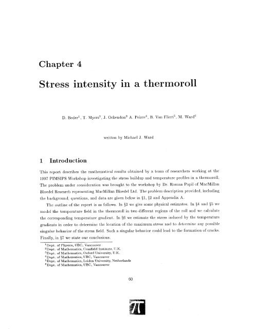
This report describes the mathematical results obta<strong>in</strong>ed by a team of researchers work<strong>in</strong>g at the<br />
1997 PIMSIPS Workshop <strong>in</strong>vestigat<strong>in</strong>g the stress buildup and temperature profiles <strong>in</strong> a <strong>thermoroll</strong>.<br />
The problem under consideration was brought to the workshop by Dr. Roman Popil of MacMillan<br />
Bloedel Research represent<strong>in</strong>g MacMillan Bloedel Ltd. The problem description provided, <strong>in</strong>clud<strong>in</strong>g<br />
the background, questions, and data are given below <strong>in</strong> §1, §2 and Appendix A.<br />
The outl<strong>in</strong>e of the report is as follows. <strong>In</strong> §3 we give some physical estimates. <strong>In</strong> §4 and §5 we<br />
model the temperature field <strong>in</strong> the <strong>thermoroll</strong> <strong>in</strong> two different regions of the roll and we calculate<br />
the correspond<strong>in</strong>g temperature gradient. <strong>In</strong> §6 we estimate the stress <strong>in</strong>duced by the temperature<br />
gradients <strong>in</strong> order to determ<strong>in</strong>e the location of the maximum stress and to determ<strong>in</strong>e any possible<br />
s<strong>in</strong>gular behavior of the stress field. Such a s<strong>in</strong>gular behavior could lead to the formation of cracks.<br />
F<strong>in</strong>ally, <strong>in</strong> §7 we state<br />
our conclusions.<br />
1Dept. of Physics, UBC, Vancouver<br />
2Dept. of <strong>Mathematics</strong>, Cranfield <strong>In</strong>stitute, U.K.<br />
3Dept. of <strong>Mathematics</strong>, Oxford University, U.K.<br />
4Dept. of <strong>Mathematics</strong>, UBC, Vancouver<br />
SDept. of <strong>Mathematics</strong>, Leiden University, Netherlands<br />
6Dept. of <strong>Mathematics</strong>, UBC, Vancouver
2 Background<br />
Dur<strong>in</strong>g the manufacture of coated paper products, a paper-mak<strong>in</strong>g stock consist<strong>in</strong>g of water and<br />
1% or less wood fibers is prepared by chemically or mechanically separat<strong>in</strong>g the fibers from wood.<br />
A screen<strong>in</strong>g process removes most of the water; the rema<strong>in</strong>der is removed through press<strong>in</strong>g aga<strong>in</strong>st<br />
felts and contact dry<strong>in</strong>g. The web is further densified by pass<strong>in</strong>g it through high pressure calender<br />
rolls, result<strong>in</strong>g <strong>in</strong> about a two-fold decrease <strong>in</strong> caliper of the pressed and dried paper. The web may<br />
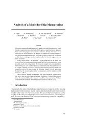
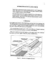
then pass through a number of calender nips. The geometry for one such nip is shown <strong>in</strong> Fig. l.<br />
This last stage of densification <strong>in</strong>volves high temperatures and pressures that lead to high stresses<br />
<strong>in</strong> the roll material.<br />
A stack consists of two rolls: one has a polymeric elastomer cover<strong>in</strong>g, the other is a solid iron alloy<br />
(the <strong>thermoroll</strong>). It is our task to estimate the stresses <strong>in</strong> the <strong>thermoroll</strong> under standard operat<strong>in</strong>g<br />
conditions, and determ<strong>in</strong>e whether it is possible, under certa<strong>in</strong> conditions, for crack<strong>in</strong>g or roll failure<br />
to occur.<br />
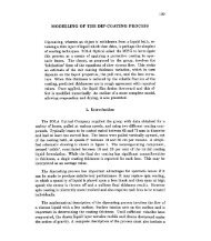
The <strong>thermoroll</strong> consists of a hollow cyl<strong>in</strong>der, rigidly attached at either end to a rotat<strong>in</strong>g bear<strong>in</strong>g.<br />
It is hydraulically loaded to 350kN /m, lead<strong>in</strong>g to a deflection at its center of l.6mm. The roll has<br />
<strong>in</strong>ner and outer radii of 560 and 750mm, respectively. It conta<strong>in</strong>s 45 bore holes with radii 16mm.<br />
Oil, heated to a temperature of 253°C, flows through these boreholes at a rate of 33.7 L/s with an<br />
energy <strong>in</strong>flux of approximately 800kW. As noted by Dr. Roman Popil, the temperature on the <strong>in</strong>ner<br />
bores may be a little different from the oil temperature and is typically an unknown quantity. We<br />
label the bore temperature as nore <strong>in</strong> the analysis below. The typical configuration is shown <strong>in</strong><br />
Fig. 1 and 2.<br />
The <strong>thermoroll</strong> is made by a cast<strong>in</strong>g process such that the outer layer, the so-called 'chill" , hav<strong>in</strong>g<br />
cooled first upon contact with the walls of the mold, imparts a residual radial stress <strong>in</strong>to the roll.<br />
The thermal and elastic properties of the chill are different from that of the bulk material.<br />
The web enters the nip at a temperature of 66°C, typically travel<strong>in</strong>g at 18m/sec. Its temperature,<br />
measured some distance from the nip, <strong>in</strong>creases by approximately 26°C.<br />
Periodically the polymer covered roll is washed, provid<strong>in</strong>g a source for dripp<strong>in</strong>g water. This may<br />
fall onto the iron roll and subsequently evaporate or 'jump" off the hot surface (and so have little<br />
effect on heat transfer).<br />
A number of sources for stress build-up <strong>in</strong> this system are easily identified, for example:<br />
• Large temperature gradients (and consequently thermal stresses) will occur <strong>in</strong> the vic<strong>in</strong>ity of<br />
the nip.
nip region where<br />
contact occurs<br />
• 92°C<br />
Figure 1:<br />
morolls.<br />
oil<br />
boreholes<br />
253°C<br />
{,iI =700mm<br />
'surf =750mm<br />
'chill=738mm<br />
I<br />
I<br />
/<br />
/<br />
/<br />
/<br />
I<br />
: a<br />
\<br />
\<br />
\<br />
\<br />
\, ,,<br />
Figure 2: Schematic plot of geometry simplified.<br />
• The iron roll manufactur<strong>in</strong>g process will <strong>in</strong>variably lead to built-<strong>in</strong> stresses (estimated by the<br />
manufacturers to have compressive radial stress components of 150 MPa).<br />
• Another compressive stress field, transmitted through the web, due to the roll's weight and<br />
load<strong>in</strong>g.<br />
• What will be the total stress <strong><strong>in</strong>tensity</strong> (residual, thermal, load<strong>in</strong>g ...) <strong>in</strong>duced dur<strong>in</strong>g this<br />
process?<br />
• Are there conceivable operat<strong>in</strong>g conditions under which the stresses could become high enough<br />
to cause crack<strong>in</strong>g, or even worse for catastrophic failure to occur?<br />
4 Physical Estimates<br />
We first estimate whether the energy <strong>in</strong>put from the oil boreholes and the quoted temperature difference<br />
across the roller are consistent. Specifically, we would like to estimate the surface temperature<br />
of the roller.
As will be shown <strong>in</strong> §4, the perturb<strong>in</strong>g effect of the nip on the rapidly rotat<strong>in</strong>g drum is small<br />
except near the nip. Thus, we can approximate the temperature <strong>in</strong> the annular iron drum between<br />
the oil boreholes and the outer surface as the radial function<br />
The values for roil and rsurj are given <strong>in</strong> Appendix A, and are roil = 700mm and rsurj = 750mm,<br />
respectively. The boundary condition T = Tbore at l' = roil determ<strong>in</strong>es one relation between A and<br />
B while the other relation is found from the given total heat flux <strong>in</strong>to the roller from the oil, which<br />
was quoted<br />
<strong>in</strong> §2. We estimate<br />
dQ<strong>in</strong><br />
~ = 27fToilKTrLroll = P on l' = rsurj .<br />
Here P is the total heat flux and Lroll is the length of the roller. Us<strong>in</strong>g the data provided, and<br />
tak<strong>in</strong>g K as that for iron, we estimate B = 39SoC. This <strong>in</strong>dicates a temperature difference between<br />
the borehole radius and the outer surface of<br />
Us<strong>in</strong>g a more ref<strong>in</strong>ed calculation, tak<strong>in</strong>g <strong>in</strong>to account the different values of the thermal diffusivity<br />
K for the chill and the core, we estimate a temperature difference of 32°C. <strong>In</strong> §5 below, we use the<br />
surface temperature of 192°C as measured by MacMillan Bloedel.<br />
Next, we estimate the heat flux and temperature gradient <strong>in</strong> the roller surface just below the<br />
nip. With a specified nip width of 1.1cm and the heat flow to the web, the estimated radial heat<br />
flux
a droplet lifetime of the order of 1 second whereas MacMillan Bloedel has estimated the "Leidenfrost<br />
thermal flux lower limit" as <strong>in</strong>put <strong>in</strong>formation.<br />
We now consider a simple scenario. Suppose that we have a hemispherical droplet of radius a,<br />
where a = 6.2mm. The required latent heat to evaporate the droplet is Clat = 2.25610 6 J Ikg. Thus,<br />
the estimate of the heat flux ¢ <strong>in</strong>to the droplet across a small patch of roller surface under the<br />
droplet is<br />
¢ = ~ (a3p~at) = 2apClat .<br />
3tdrop 7ra~ 3tdrop<br />
Us<strong>in</strong>g the estimates a = 6.2mm and the droplet lifetime tdrop = lsec, we get an estimate ¢ =<br />
l07w 1m 2 , which is four times larger than the heat flux estimated from the nip region. It therefore,<br />
appears crucial to do a careful analysis of temperature gradients and the result<strong>in</strong>g stress field near<br />
the droplet. This analysis is very difficult and was not done by our group.<br />
<strong>In</strong> this section we calculate the temperature field <strong>in</strong> the region away from the nip to determ<strong>in</strong>e the<br />
effect of the oil bores on the heat<strong>in</strong>g of the drum. This is referred to as the global problem. <strong>In</strong><br />
this problem, the nip region is replaced by a po<strong>in</strong>t s<strong>in</strong>k of strength Q. The strength of this s<strong>in</strong>k can<br />
be determ<strong>in</strong>ed by the estimate obta<strong>in</strong>ed <strong>in</strong> §3.<br />
It is convenient <strong>in</strong> the analysis to fix ourselves <strong>in</strong> a frame <strong>in</strong> which the thermo roll is stationary<br />
and the nip region on the edge of the <strong>thermoroll</strong> is rotat<strong>in</strong>g at an angular velocity w = vll's1l1·.t. The<br />
mathematical model for the temperature field T, where T is measured <strong>in</strong> °C, is<br />
(7a)<br />
(7b)<br />
(7 c)<br />
Here k ch is the thermal diffusivity of the chill and {)is the Dirac delta function. The parameter", <strong>in</strong><br />
(7a) is piecewise constant, with", = "'ch <strong>in</strong> the chill region rchill < r < rSllrj, and", = "'co <strong>in</strong> the core<br />
region roil < r < r chill. The values for these constants are given <strong>in</strong> Appendix A. As a simplify<strong>in</strong>g<br />
approximation to the geometry, <strong>in</strong> this model we have replaced the <strong>in</strong>dividual boreholes by a l<strong>in</strong>e of<br />
boreholes along r = roil. Although such an approximation should warrant further study, it greatly<br />
simplifies the analysis. <strong>In</strong> this model we have also assumed a negligible heat transfer between the<br />
air and the <strong>thermoroll</strong>. <strong>In</strong> a more ref<strong>in</strong>ed analysis than is presented below, a Newtonian cool<strong>in</strong>g<br />
boundary condition should be imposed on the edge of the <strong>thermoroll</strong>.<br />
There are two goals to the analysis below. Firstly, we would like to justify why the temperature<br />
can be approximated by a radially symmetric function away from the nip region. Secondly, we would<br />
like to estimate the temperature gradient as we approach the nip region.
We <strong>in</strong>troduce non-dimensional variables by p = r / r sur j and T = t / w. The non-dimensional<br />
rotation<br />
rate Wn is def<strong>in</strong>ed by<br />
We estimate that Wn = 10 6 , which is very large. This value measures the importance of rotation<br />
as compared to thermal diffusion, and can be thought of as a Peclet number. The non-dimensional<br />
model is<br />
(9a)<br />
T(po,O,t)<br />
Tp(l, 0, t)<br />
(9b)<br />
(9c)<br />
Here Po == roil/rsurj, Q = Qrsurj/Koh, while k = 1 <strong>in</strong> the chill region and k = Kco/Koh <strong>in</strong> the core.<br />
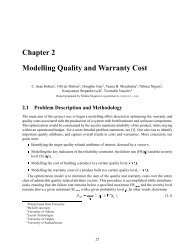
A schematic plot of the geometry is shown <strong>in</strong> Fig. 3.<br />
We look for a solution to (9) <strong>in</strong> the form<br />
(l1a)<br />
(l1b)<br />
(l1c)<br />
Next, we seek a solution to (11) <strong>in</strong> the rapid rotation limit Wn ~ 1. <strong>In</strong> the outer region, def<strong>in</strong>ed<br />
away from the nip near ¢ = 0, we substitute<br />
the expansion<br />
I<br />
F(p, ¢) = Fo(p, ¢) + -F 1 (p, ¢) + ... ,<br />
W n<br />
0,<br />
_k- l F 1 ¢, Po < p < 1.<br />
(13a)<br />
(13b)<br />
S<strong>in</strong>ce F 1 is periodic <strong>in</strong> ¢, it follows that f~7r F1¢d¢ = 0. Therefore, upon <strong>in</strong>tegrat<strong>in</strong>g (13b), we<br />
obta<strong>in</strong> that Fa satisfies
.0-8 -0<br />
/3 U.<br />
o 6)<br />
53 Q<br />
:: ~urf q "<strong>In</strong>ner" nip<br />
~ CD<br />
CD<br />
o ~il (£)<br />
~ ,d<br />
'G /0 ,- -<br />
- 0,' Heat s<strong>in</strong>k for<br />
I<br />
I -/<br />
P<br />
nip region<br />
One boundary condition for Fa is Fa = nore at P = Po. There are two possible conditions that<br />
can be imposed for the second relation. One choice would be to specify the flux out of P = Po as <strong>in</strong> §3,<br />
which would determ<strong>in</strong>e B. The second choice would be to satisfy the boundary condition Fop = O.<br />
Note that a better approximation to the boundary condition would be to impose a Newtonian<br />
cool<strong>in</strong>g condition on the surface of the roller characterized by some Biot number, represent<strong>in</strong>g a<br />
heat transfer coefficient between the air and the chill. Specify<strong>in</strong>g the flux out of the boreholes would<br />
enable us to calculate this coefficient. The temperature field, away from the nip region, is obta<strong>in</strong>ed<br />
by substitut<strong>in</strong>g (14) <strong>in</strong> (10).<br />
Our first conclusion is that <strong>in</strong> the limit of rapid rotation the temperature field away from a th<strong>in</strong><br />
zone near the nip region is radially symmetric.<br />
The solution (14) is not valid <strong>in</strong> the vic<strong>in</strong>ity of the nip region where ¢ = O. Thus, as is usual <strong>in</strong><br />
s<strong>in</strong>gular perturbation problems, we must construct an <strong>in</strong>ner solution near ¢ = 0, p = 1. The extent<br />
of this region is O(w;;-l). We <strong>in</strong>troduce the local variables p and ¢ by<br />
-F¢ Fpp+F¢¢, O
$=0<br />
)<br />
<strong>In</strong>ner nip<br />
regionis<br />
magnified to<br />
__<br />
Here Ko(z) is the modified Bessel function of the first k<strong>in</strong>d of order zero. <strong>In</strong> terms of the orig<strong>in</strong>al<br />
variables,<br />
we have<br />
Therefore, us<strong>in</strong>g the asymptotic behavior of Ko(z), we observe that as we approach the nip region<br />
the change <strong>in</strong> temperature !:::,T = T - 192 behaves logarithmically like<br />
Here Q is the strength of the heat s<strong>in</strong>k. Thus, for the global problem the temperature decrease as<br />
we approach the nip region is only logarithmic with the distance from the nip. The effect of the<br />
result<strong>in</strong>g temperature gradient on the stress field is estimated <strong>in</strong> §6.<br />
We now calculate the temperature field <strong>in</strong> the region near the nip. This is referred to as the local<br />
problem. <strong>In</strong> the near-nip region, the geometry is approximately planar as shown <strong>in</strong> Fig. 5. The<br />
contact region between the paper and the roller is approximately 2cm as shown <strong>in</strong> this figure. The<br />
goal is to estimate the temperature gradients near the lead<strong>in</strong>g edge where the paper first comes<br />
<strong>in</strong>to contact with the roller (see the figure). It is <strong>in</strong> this region that we expect the temperature<br />
gradients to be largest. Note that the calculations below are done <strong>in</strong> a frame for which the lead<strong>in</strong>g<br />
edge is located at X = 0 (see Fig. 5).<br />
From the data given <strong>in</strong> Appendix A, the values for the thermal diffusivity of the water Kw, the<br />
chill Kch and the core Kco are
From these values, we can estimate a Peclet number, which is a dimensionless parameter giv<strong>in</strong>g a<br />
measure of the relative strengths of convection compared to the thermal diffusion. S<strong>in</strong>ce Pe = vL/ K,<br />
we can estimate a Peclet number us<strong>in</strong>g v = 18m/see, L = 2cm, and K = 0.lcm 2 /sec to get Pe =<br />
18000, which is very large. Hence the temperature field near the nip is dom<strong>in</strong>ated by convection.<br />
We now formulate the model. We approximate the temperature field <strong>in</strong> the near nip region us<strong>in</strong>g<br />
a steady-state convection-diffusion equation<br />
where we take L = 2cm and Pe = VL/Kch. <strong>In</strong> terms of these variables, the length of the contact<br />
region between the paper and the roller is extremely large and thus, as a good approximation, we<br />
take the contact region to be of semi-<strong>in</strong>f<strong>in</strong>ite extent occupy<strong>in</strong>g the region .r < 0, Y = 0. <strong>In</strong> terms of<br />
these new variables, the chill region extends very deeply below the contact region and hence we will<br />
take the chill to occupy the region below the x-axis.<br />
We now formulate the boundary conditions. The l<strong>in</strong>e x > 0, Y = ° is where the roller is exposed<br />
to the air and hence we assume that there is negligible heat transfer between these two media (i.e.<br />
T y = ° for x > 0, Y = 0). This assumption should be exam<strong>in</strong>ed more carefully <strong>in</strong> a more ref<strong>in</strong>ed<br />
analysis. <strong>In</strong> addition, we assume that the temperature field and the heat ft.ux are cont<strong>in</strong>uous across<br />
the contact region.<br />
Next, we give far field conditions for the temperature field. The surface temperature of the roller<br />
obta<strong>in</strong>ed from the global problem is estimated by MacMillan Bloedel Research to be T = 192°C. This<br />
yields the asymptotic match<strong>in</strong>g condition T -> 192°C as y -> -00. F<strong>in</strong>ally, the web temperature<br />
<strong>in</strong>to the nip is 66°C and thus we set T -> 66°C as y -> +00.
To summarize, the model for the temperature field <strong>in</strong> the near nip region (see Fig. 6), where T<br />
is measured <strong>in</strong> 0 C is<br />
(23a)<br />
(23b)<br />
T+y(x,O)<br />
T+(x,O)<br />
T+<br />
T_y(x,O) = 0 for x> 0<br />
T_(x,O); 6T+y(x,0) = T_y(x,O) for x 0, (28a)<br />
uOfj(x,O) 0 for x> 0; uo(x, 0) = 192 for x < 0, (28b)<br />
Uo<br />
-7<br />
66 as y -7 +00. (28c)<br />
(29a)<br />
(29b)
8 T = T ---...<br />
+y -y ~ T =T =0<br />
+y -y<br />
T =T 1<br />
+ -~<br />
~y<br />
uo- = 0<br />
y<br />
paper<br />
regIOn<br />
To get a well-posed problem, we solve (28) <strong>in</strong> the region x < 0, with the "<strong>in</strong>itial" condition<br />
uo(O, fj) = 192. The solution is readily found to be<br />
uo(x,fJ) = 66+ 126 Erfc (fJ/2(-x)1/2) ,<br />
where Erfc(z) is the complementary error function. Thus, the isotherms occur along the curves<br />
fj = C(_X)1/2 for c> 0 and x < 0 (see Fig. 7). A simple calculation then yields<br />
126<br />
uOfj(x,0)=-(_?rx)1/2' for x
G(x'; x) = - 2~ e(X'-x)/2 [K o (Ix' - xl) + K o (Ix' - x* I)) .<br />
132]00 1 , I '<br />
v(x,y) = - Vif -00 V_x,G(x ;x) y'=odx .<br />
Substitut<strong>in</strong>g (30) and (34) <strong>in</strong>to (26) and (27) yields the temperature profile <strong>in</strong> the web and the chill<br />
regions, respectively. It is easy to show that the limit<strong>in</strong>g behavior of v as we approach the lead<strong>in</strong>g<br />
edge is<br />
where C = -252/Vif.<br />
The solution for T_ <strong>in</strong> the paper becomes <strong>in</strong>valid <strong>in</strong> an 0(8) neighborhood oflead<strong>in</strong>g edge. This<br />
follows from the fact that we have neglected the diffusion term T- xx <strong>in</strong> obta<strong>in</strong><strong>in</strong>g (28). Hence we<br />
need an <strong>in</strong>ner-<strong>in</strong>ner region where x = 0(8) and y = 0(8). <strong>In</strong>troduce the new variables<br />
(38a)<br />
o for x> 0;<br />
66 as fJ -> +00 .<br />
(38b)<br />
(38c)<br />
(39a)<br />
(39b)<br />
The solution v must match with the behavior (35) <strong>in</strong> the far field.<br />
by<br />
The solution to (38) can be found explicitly <strong>in</strong> terms of the parabolic coord<strong>in</strong>ates ~ and 7] def<strong>in</strong>ed<br />
A_I (.
<strong>In</strong> terms of these coord<strong>in</strong>ates the problem (38) reduces to the follow<strong>in</strong>g ord<strong>in</strong>ary differential equation<br />
problem<br />
for u(1]):<br />
Us<strong>in</strong>g the def<strong>in</strong>ition of the change of coord<strong>in</strong>ates we can calculate the derivative needed <strong>in</strong> the<br />
problem<br />
(39) for v. We get<br />
'(A 0) 126 ~<br />
u x, = - (-71"X )1/ 2 ' 101' X < 0,<br />
and r= ' (A2 x + y A2)1/2 .<br />
Substitut<strong>in</strong>g (44) <strong>in</strong>to (37) determ<strong>in</strong>es the temperature field <strong>in</strong> the chill region of the <strong>thermoroll</strong> <strong>in</strong><br />
the immediate vic<strong>in</strong>ity of the lead<strong>in</strong>g edge where the paper first makes contact with the roller.<br />
The ma<strong>in</strong> conclusion from this analysis is that this temperature field near the lead<strong>in</strong>g edge has<br />
the behavior<br />
for some constant B. Thus, it has an <strong>in</strong>f<strong>in</strong>ite gradient of square-root type at the lead<strong>in</strong>g edge. <strong>In</strong><br />
§6 we estimate whether this s<strong>in</strong>gular form leads to a s<strong>in</strong>gular stress field at the lead<strong>in</strong>g edge.<br />
We now estimate the stress field <strong>in</strong>duced by the temperature gradients calculated <strong>in</strong> §4 and §5. We<br />
will consider both the local and the global problems.<br />
The equilibrium equation from elasticity theory for the displacement vector u is<br />
3(1- v) "V ("V. u) _ 3(1- 2v)"V x "V xu = o:"VT.<br />
(l+v)<br />
2(1+v)<br />
Here v is Poisson's ratio, o:"VT is the body force <strong>in</strong>duced by the thermal gradient, and 0: is a constant.<br />
The stress tensor CTij is determ<strong>in</strong>ed <strong>in</strong> terms of u by
Here>' and G are the Lame' constants. Thus, the stress is (essentially) proportional to the first<br />
derivatives of u.<br />
Consider the local problem for which the temperature field behaves like (45) at the lead<strong>in</strong>g<br />
edge. Then decompos<strong>in</strong>g V'u <strong>in</strong> terms of a radial component Ur and an angular component Ue, we<br />
get the follow<strong>in</strong>g equations from (46):<br />
3(1- v) (orrur + ... ) _ 3(1- 2v) (Oreue + ...) = 0: ( C,) s<strong>in</strong> (~) ,<br />
(l+v) 2(1+v) l' 21'2 2<br />
_3(_1-_v_)(_or_eu_r+ ...) + _3(_1_-_2v_) (orrue + ... ) = -0: (_C_,) cos (~)<br />
(1+v) l' 2(1+v) 21'2 2<br />
From these equations, a simple dom<strong>in</strong>ant balance argument shows that the two components satisfy<br />
u,. = 0(1'3/2) and ue = 0(1'3/2) as l' -+ o. Thus the stress field has the form<br />
Hence the stress field is not s<strong>in</strong>gular at the lead<strong>in</strong>g edge, and there is no significant stress <strong>in</strong>tensification,<br />
such as that determ<strong>in</strong>ed by a stress <strong><strong>in</strong>tensity</strong> factor. <strong>In</strong> fact, the stress field behaves like<br />
that for a contact problem (i.e. a Barenblatt "crack").<br />
Now consider the global problem where the nip region is approximated by a delta function. The<br />
geometry is shown <strong>in</strong> Fig. 4 and the temperature field has the behavior given <strong>in</strong> (19). Substitut<strong>in</strong>g<br />
T ~ <strong>In</strong> l' <strong>in</strong>to (46) we can obta<strong>in</strong> the behavior of u,. us<strong>in</strong>g a dom<strong>in</strong>ant balance argument. We<br />
estimate o,.u r = O(ln 1') and hence the radial component of the stress is (J"r = O(ln 1'). Thus, the<br />
stress field grows logarithmically <strong>in</strong> the outer region but is then cut off as we approach the <strong>in</strong>ner<strong>in</strong>ner<br />
region. Once aga<strong>in</strong>, we conclude that there is no significant <strong>in</strong>tensification of the stress, such<br />
as that determ<strong>in</strong>ed by a square root s<strong>in</strong>gularity for which a stress <strong><strong>in</strong>tensity</strong> factor can be def<strong>in</strong>ed.<br />
The ma<strong>in</strong> focus of our group was to calculate the temperature gradient <strong>in</strong> the <strong>thermoroll</strong> and to<br />
determ<strong>in</strong>e whether this gradient can lead to an <strong>in</strong>tensification of stress <strong>in</strong> the nip region.<br />
The temperature gradient was calculated for both a global temperature model <strong>in</strong> which the nip<br />
is represented by a po<strong>in</strong>t source and a local temperature problem, def<strong>in</strong>ed <strong>in</strong> the vic<strong>in</strong>ity of the<br />
nip region, where we studied <strong>in</strong> detail the region where the paper first comes <strong>in</strong>to contact with the<br />
roller. For both the local and global temperature problems we calculated the s<strong>in</strong>gular behavior of<br />
the thermal field. <strong>In</strong> §6, we used the s<strong>in</strong>gular behavior of the thermal field <strong>in</strong> a model to estimate<br />
the stress field for both the local and global problems. The goal was to ascerta<strong>in</strong> whether such<br />
a temperature gradient can lead to a s<strong>in</strong>gular stress field. Such a stress field is known <strong>in</strong> other<br />
circumstances to <strong>in</strong>duce crack formation. Our conclusion <strong>in</strong> §6 is that the stress field is not s<strong>in</strong>gular
for either the local or global problems, and hence, from our model of the <strong>thermoroll</strong>, the temperature<br />
gradients are not likely to be the cause of roll fracture.<br />
We also showed that <strong>in</strong> the limit of large drum rotation, which is the usual operat<strong>in</strong>g regime of<br />
the <strong>thermoroll</strong>, the temperature distribution <strong>in</strong>side the <strong>thermoroll</strong> is well approximated by a radially<br />
symmetric function. This can allow for an accurate calculation of the surface temperature on the<br />
roller once a more precise boundary condition can be applied to the roller surface.<br />
F<strong>in</strong>ally, a crude physical estimate <strong>in</strong> §3 suggested that there can be extremely large temperature<br />
gradients as a result of dripp<strong>in</strong>g water onto the <strong>thermoroll</strong>. This problem certa<strong>in</strong>ly warrants an<br />
<strong>in</strong>tensive <strong>in</strong>vestigation.<br />
We are grateful to Dr. Roman Popil of MacMillan Bloedel Research Ltd. for his explanation of this<br />
problem to us and for his detailed comments on this report. We would also like to thank Dhavide<br />
Aruliah for prepar<strong>in</strong>g the figures for this paper.<br />
Web temperature out of nip = 92°C<br />
Web temperature <strong>in</strong>to nip = 66°C<br />
Web velocity<br />
= 18m/see<br />
Web width<br />
= 7770 mm<br />
<strong>In</strong>ner core radius<br />
= 560mm<br />
Outer core radius = 750mm<br />
Thickness<br />
Thickness<br />
of chill<br />
of shell<br />
Thermal conduct. chill<br />
Thermal conduct. core<br />
Bore hole radius<br />
Number<br />
Oil flow rate<br />
of bores<br />
Oil temperature<br />
= 12mm<br />
= 49mm<br />
= 24W/mK<br />
= 48W/mK<br />
= 16mm<br />
= 45<br />
= 33.7L/sec<br />
= 253°C<br />
The thermal diffusivities of the water, chill and core, which we label by /\'w, /\,ch and /\'co, respectively,<br />
are now calculated <strong>in</strong> terms of more conventional units. For water, p = 10 3 kg/m 3 ,<br />
C p = 4186 J /kg-K, k = 0.6 W/mK, and thus<br />
/\,w = k/ pCp = 0.142 X 10- 6 m 2 /sec = 0.142 x 10- 2 cm 2 /sec. (50)
Lastly, Kco = 2Kch.<br />
F<strong>in</strong>ally, we quote the estimate of the heat flow <strong>in</strong>to the web given by Macmillan Bloedel Research.<br />
For each unit length along the roll we have dmj dt = 1.1kgjs and the heat flux <strong>in</strong>to the web is<br />
Here 6T = 26°C is the temperature difference along the web. This <strong>in</strong>put estimate might be based<br />
on too much water content, and if so it would turn out that the heat <strong>in</strong>put <strong>in</strong>to the web is smaller<br />
by a factor of ten.