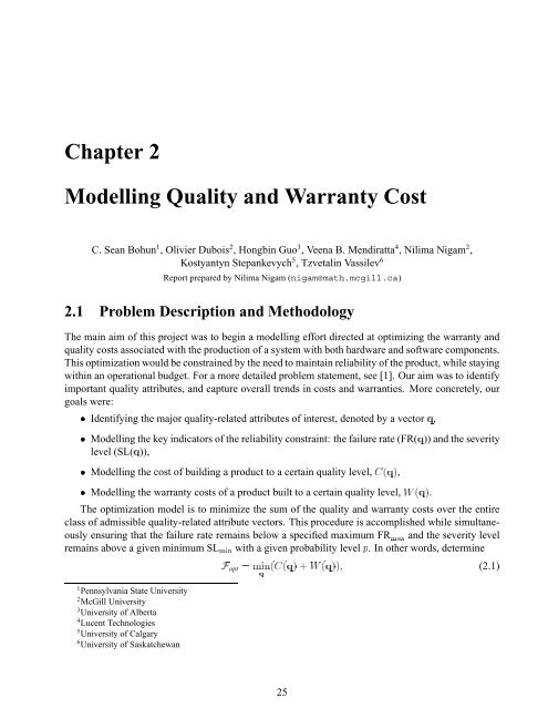
Chapter 2 Modelling Quality and Warranty Cost - Mathematics in ...

Chapter 2
Modelling Quality and Warranty Cost
C. Sean Bohun 1 , Olivier Dubois 2 , Hongbin Guo 3 , Veena B. Mendiratta 4 , Nilima Nigam 2 ,
Kostyantyn Stepankevych 5 , Tzvetalin Vassilev 6
Report prepared by Nilima Nigam (nigam@math.mcgill.ca)
2.1 Problem Description and Methodology
The main aim of this project was to begin a modelling effort directed at optimizing the warranty and
quality costs associated with the production of a system with both hardware and software components.
This optimization would be constrained by the need to maintain reliability of the product, while staying
within an operational budget. For a more detailed problem statement, see [1]. Our aim was to identify
important quality attributes, and capture overall trends in costs and warranties. More concretely, our
goals were:
r
Identifying the major quality-related attributes of interest, denoted by a vector 9 ,
Modelling the key indicators of the reliability constraint: the failure rate (FR(9 )) and the severity
level (SL(9 )),
r
Modelling the cost of building a product to a certain quality level, ä ‚9; ,
r
Modelling the warranty costs of a product built to a certain quality level, j‚9; .
The optimization model is to minimize the sum of the quality and warranty costs over the entire
class of admissible quality-related attribute vectors. This procedure is accomplished while simultaneously
ensuring that the failure rate remains below a specified maximum FR687:9 and the severity level
remains above a given minimum SL68;=< with a given probability level > . In other words, determine
1 Pennsylvania State University
2 McGill University
3 University of Alberta
4 Lucent Technologies
5 University of Calgary
6 University of Saskatchewan
opt ¥§¤ž ? ä ‚9;Lxj:95€ (2.1)
7
25

J
26 CHAPTER 2. MODELLING QUALITY AND WARRANTY COST
subject to
ê+ FR‚9;A@ FR687:9÷B@C>¸ ê+ SL:9WÆ SL68;= (2.2)
over all admissible 9 . In this project we did not perform this optimization, focusing instead on the
modelling of the function involved.
It is important to note at this juncture that no raw data from Lucent was provided for this project,
nor did we have specific information about the particular products being built. It was therefore not
feasible to use existing hazard/risk models for the various components. Our modelling effort was thus
critically dependent on discussions with the industrial contact, Prof. Veena Mendiratta. In the section
on future directions we make a series of recommendations which will help refine the models involved.
We systematically identified the key quality-related attributes, described by a quality vector 9 ,
which could be measured and quantified. We then developed reliability, warranty and cost models
based on these. As our discussions progressed, it became clear that these quality attributes were not
all independent. Nor were they all equally important indicators of overall quality. It is thus possible to
simplify the models considerably by focusing on the effects of the most important attributes, making
the optimization problem (2.1) simpler to solve. In practice, once cost functions and parameters have
been picked on the basis of standard hazard models, it will be possible via scaling arguments to achieve
further simplification.
With a view to illustrating qualitative trends predicted by our models, we generated some test data
(see Subsection 2.8), and ran our models on them. The graphs presented in this report are therefore
not linked to any true data, and serve only to provide qualitative information.
2.1.1 A Road Map
The following list details the strategy for this report. Figure 2.1 illustrates how the various sections of
the report interconnect.
Section 2: In this section we identify the quality-related variables, D , which drive the various
costs associated with a product, and over which the optimization will occur. The fact that many
of these variables are not independent will be dealt with later in this report.
Section 3: Here, we develop models for the reliability constraints, the failure rate FR and the
severity levels SL. As well as providing some graphical insight into the dependence of these
models on the quality D , we also discuss how these failure rates determine the probability of the
various modes of failure. These probabilities play a role in determining the warranty costs of a
product.
Section 4: At this point in the report a model EGFDIH for , the cost of implementation of a given
quality D level is proposed.
Section 5: This contains the development of the warranty models for J hardware
sw aspects of a product.
hw and software
Section 6: Here we combine the models to summarize the total proposed optimization problem.
Section 7: A sensitivity to parameters is discussed, providing insight into the relative importance
of terms in the various models that have been introduced.

S
УÑÓÒÕÔWÖ×ÙØnÚMÛÝÜÞ×àß
á£âÓãÕäWå5æç¤åéèÝê
ë£ìÓíÕîWï5ðñnò¡óÝôWõ
2.2. QUALITY ATTRIBUTES VECTOR 27
/.0
XWLTYZV QR[
KML¤N¤L¤OP¤QRLBPTS¤L¤UWV
f gRhMij_kgRa¤\
\]_^¤`¤a¤b&c¤d¤]¤e
¢¤ ¢!#"%$'&)(+*
¢¡¤£¦¥¨§©
1.2
3.4.576
lnm¤op¤qZm¤or
sut¤vRwRxZy¤z{
=.?A@
Ã5Ä¤Å Æ Ç¤ÈÉBÈĤÊRÉÌËÃÎÍÏ
|n}8|¤~T|¤T|¤€
¤‚T¤ƒT¤„B¤…T¤†
u·¤¸W·¤¹º »R¼M½ ·¤¸W·¤½¿¾ ÁÀ¡Â
,.-
‡Mˆ¤‰¤Š ‹ ŒR
ö£÷ÓøÕùWú5ûü¤úMýþ¿ÿ
8.9.:7;
B.C.DAE
§n¨¤©ª¤«Z¨¤©¬T«Z¨¤©©¨_­¤®R¯¡° ±³²:´+µ
–$—¤˜RRšZ›¤œTšZ›¤œœ›¤ž¤RŸ¡ ¢©£¥¤+¦
FG
ŽW¤R‘¤’W“”¤•W
Figure 2.1: Illustrated are the various sections of this report and how they interconnect.
Section 8: Broad trends in the proposed models are generated by drawing the quality-related
variables from a given probability distribution. Two cases are considered, each characterized by
the probability distribution being used.
2.2 Quality Attributes Vector
We begin by identifying the important quality-related attributes which are both salient and measurable
in the context of this project. These attributes fall into two broad categories – hardware-related and
software-related – and the optimization of the total cost will be performed over these attributes. In
practice, most of these attributes will be measured statistically. In the absence of raw data, we are
unable to provide statistical models for these attributes, which will change depending on the product.
Mathematically, these attributes are gathered in a quality vector
K.LMJON#L JOP#LMQQQRLMJTSHVUXWZYRH\[^]L)_` Q
DIH4F7J
The cost will be optimized as a function DaUbW of , subject to certain reliability constraints. We
have scaled these J>c attributes to take on values between 0 and 1 for convenience. This enables us to
compare, for example, a quantity originally measured as a percentage with one measured as a number
between 0 and 10. When using the model in application, it will be important to identify the units used
and convert them if necessary.
The various quality attributes are described below.
HARDWARE:
: Component quality. In practice measured as a failure rate percentage per year. Here, this rate is
JMK
converted to a scale from 0 to 1, and is JMK called .

r
28 CHAPTER 2. MODELLING QUALITY AND WARRANTY COST
: Infant mortality factor (IMF). Measured as the ratio of the initial failure rate to the steady-state
JON
failure rate, this is a number between 1 and 2. In this project, we use the JONdH scaling measured
infant mortality ef_ factor .
: Diagnostics capability. This attribute is denoted JOP and lies between 0.8 and 1. In practice, it is
JOP
measured as a percentage, typically between 80 and 100.
: Working environment range. The variable JTg is defined as the amount by which the constructed
JOg
working range exceeds the specifications of the device. For example, suppose the device is intended
to operate ]ih between C _])]ih and C, but is built with a working range ej_]ih of C _k)lih to C.
The constructed working range exceeds the operational specifications _]ih by C on the lower end,
and k)lih by C on the higher end. Thus, we would JOgmH compute
From the description of these hardware-related attributes, it is not immediately obvious which are the
best indicators of overall quality.
l)qs_])]tHu])Q
l .
FO_]onpk)lH>qF working rangeHoH
SOFTWARE:
: Software development environment (SDE). Denoted JTv , this describes the overall quality metric
JOv
of the software development process.
: Code complexity. This metric measures the complexity of a code based on a variety of indicators.
JOw
Essentially, the more complicated the interactions between different parts of a large code, the
harder it is to ensure reliability.
: Stability index. Typically a number between 0.8 and 1, this metric describes the robustness of a
JMx
code over longer periods of time.
: Coverage testing. This attribute describes how comprehensively each module of the code has
JOy
been checked.
: Fault density. This measures the number of failures per 1000 lines of code. We express this as a
JOS
fraction between 0 and 1.
The SDE index clearly seems to include, or be affected by, the other software-related attributes. We
expect a good model will therefore be very sensitive to changes in JOv . In particular cases, these quality
attributes may be restricted to tighter “operating ranges” by the company’s production policies.
2.3 How do we Model the Reliability Constraints?
The optimization of the costs of quality and warranty would be straightforward in the absence of
certain reliability constraints. These constraints are identified as benchmarks, or standards, which
must be met by any product. The quality attributes must be chosen to meet or exceed these standards.
Prior to prescribing the nature of the constraints, we need to model the indicators of reliability
which will be used. There are two major indicators, one for hardware and one for software.

2.3. HOW DO WE MODEL THE RELIABILITY CONSTRAINTS? 29
HARDWARE:
Failure Rate (FR): this is described by the system failure rate per year, and includes the
effect of the component failure rate J K .
SOFTWARE:
Severity Levels (SL): ranges in scale from 1 to 4, where SL Hz_ is a catastrophic failure,
and SL H|{ is a minor error.
The reliability constraints will be interpreted in terms of these indicators – the failure rate FR must be
below a certain prescribed value with high probability, and the severity level SL must stay away from
the catastrophic failures with high probability. This is illustrated in expression (2.2).
2.3.1 Modelling the Failure Rate
The failure rate used in the characterization of reliability combines several factors including the failure
rate of the components themselves, the robustness of the overall architecture, the infant mortality factor
(IMF) and the working environment range.
We identified the broad trends that the failure rate exhibited in three of the quality attributes: component
failure rate JMK , the infant mortality factor JON and the working environment range JOg . As the
component failure rate JMK increases, so does the overall failure rate. Likewise, if the IMF JTN is high,
the failure rate is large. The effect of the working range environment JOP is opposite: if the constructed
working range is larger than the specs, the device is more robust and thus the failure rate goes down.
We proposed two models with increasing complexity that exhibit this behaviour. Our discussions
revealed that in this specific context the failure rate was described largely in terms of the component
quality.
The first model FRK_FDMH is a simple one, with 3 free parameters }~K , }N , and }P :
FRKFDIHH FRK¤F7JMK.L JON#LMJTgHH€})KsJ K n‚}NƒJON„e…}PuFO_e…JMKH>JOgQ (2.3)
The nonlinear term e†}PuF>_‡e€JMKH>JOg enters since the failure rate should decrease with larger working
environment range JTg , however the system will nevertheless be affected by poor component failure
rates J K . These two effects are therefore competing.
Figure 2.2 below shows four graphs related to failure rate model FRK . The first three graphs exhibit
the trends of the failure rate with respect to the individual attributes JMK , JTN , JOg . The last graph depicts a
surface plot describing failure rate trends when J K and JOg are allowed to change.
The next failure rate model we propose is manifestly nonlinear, and aims to better capture the
importance of the component failure rate J K on the system failure rate FR. The free parameters are
denoted }~K , }N , }P and }g . As before, the failure rate FR depends on the quality vector D , but in
particular on the attributes JMK , JTN , JOg .
N
e…}guFO_e…JMKH>JOgQ (2.4)
K
K>LMJTNLMJOg_HVH|})Ksˆ¦‰¦ŠŒ‹.Žn…}P JONMJ
FRNuF7J
The rationale for picking this model is as follows: first, the system failure FRF DMH rate increases with
poorer component quality, with this rate of change depending JMK on . Therefore the dependence of

30 CHAPTER 2. MODELLING QUALITY AND WARRANTY COST
0.24
FR1 v/s q1, q2=0.3
0.5
FR1 v/s q2, q4=0.3
0.22
0.2
0.4
0.18
0.16
0.3
0.14
0.12
0.2
0.1
0.08
0.06
q4=0.1
q4=0.5
q4=0.8
0.1
q1=0.1
q1=0.5
q1=0.8
0.04
0 0.1 0.2 0.3 0.4 0.5 0.6 0.7 0.8 0.9 1
Component Failure Rate q1
0.25
(a)
FR1 v/s q4, q4=0.3
0
0 0.1 0.2 0.3 0.4 0.5 0.6 0.7 0.8 0.9 1
Infant Mortality Factor q2
(b)
q1=0.1
q1=0.5
q1=0.8
1
0.9
0.22
0.2
0.8
0.2
0.15
0.1
Working Environment Range
0.7
0.6
0.5
0.4
0.3
0.2
0.18
0.16
0.14
0.12
0.1
0.08
0.05
0 0.1 0.2 0.3 0.4 0.5 0.6 0.7 0.8 0.9 1
Working Environment Range q4
(c)
0.1
0
0 0.1 0.2 0.3 0.4 0.5 0.6 0.7 0.8 0.9 1
Component Failure Rate
(d)
0.06
Figure 2.2: Failure Rate FRK model as a function of (a) component J K quality , (b) infant JON mortality ,
(c) working environment JOg range , and (d) JMK both JTg and JTNdH|]Q
together, .

2.3. HOW DO WE MODEL THE RELIABILITY CONSTRAINTS? 31
0.25
FR2 v/s q1, q2=0.3
0.25
FR2 v/s q2, q4=0.3
q1=0.1
q1=0.5
q1=0.8
0.2
0.2
0.15
0.15
0.1
q4=0.1
q4=0.5
q4=0.8
0.05
0 0.1 0.2 0.3 0.4 0.5 0.6 0.7 0.8 0.9 1
Component Failure Rate q1
(a)
0.1
0 0.1 0.2 0.3 0.4 0.5 0.6 0.7 0.8 0.9 1
Infant Mortality Factor q2
(b)
Figure 2.3: Failure Rate model FRN as a function of (a) component quality JMK , and (b) infant mortality
JON .
on JMK is modelled by an exponential. Second, the initial mortality rate JOg impacts the overall failure
FRN
rate, but even if this IMF is low, a poor-quality component will impact the failure rate adversely.
The two graphs in Figure 2.3 use the failure model (2.4) for FR to describe the broad trends in the
model with component failure J K rate and infant mortality JON factor and can be compared to Figure 2.2.
In Section 2.8 we show the effect of inputting several instances D of , drawn from test data, into the
FRN model .
2.3.2 Modelling the Severity Level
Software failures are characterized in terms of varying severity levels (hereafter denoted SL), where
an H _ SL is a catastrophic failure, while an Hu{ SL is a minor failure. In this section we present some
models describing the relationship between the quality D vector and the SL.
In the context of this specific project, we determined that the severity levels of software failure were
impacted by the software development environment JOv , the code complexity JOw , the stability index JMx ,
the coverage testing JOy and the fault density JTS . The model we propose for the severity levels is not
an additive/linear one. We believe that the chosen functional form captures well the trends in severity
levels as functions of the individual attributes, as well as the relative importance amongst these factors.
There are some free (nonnegative) parameters in the model, ‘’K , ‘N , ‘¦P , ‘¦g , ‘¦v . The severity level SL as
a function of D is:
N
Q (2.5) x
SLK_FDIHH
SLK¤F7JOvL JOw#LMJ x.LMJOyMLMJOS_HVH|‘¢K.ˆ¦“ Š•”‹T–˜—~š
y
“>› ”‹Tœ•—~š
K
” JTv„n F>_žn…JTwŸe J
”A—
N
H¡“T¢¦J w
To describe the effects of coverage testing JOy , we noted that as JTy increases, the likelihood of
catastrophic software error decreases since more of the software is validated. Similarly, as the number
of faults per 1K lines, JTS , increases, so does the risk of catastrophic error. Keeping in mind the scale

N
32 CHAPTER 2. MODELLING QUALITY AND WARRANTY COST
4.5
Severity Level
1
Severity Levels
4.5
4
3.5
0.9
0.8
4
3
0.7
3.5
2.5
2
1.5
Code Complexity
0.6
0.5
0.4
0.3
3
2.5
2
1
0.2
1.5
0.5
0.1
0
0 0.1 0.2 0.3 0.4 0.5 0.6 0.7 0.8 0.9 1
SDE
(a)
0
0 0.1 0.2 0.3 0.4 0.5 0.6 0.7 0.8 0.9 1
SDE
(b)
1
Figure 2.4: Severity levels as a function of the various components of the quality-related vector: (a)
SDE JTv , (b) SDE and code complexity F£JOvLMJTw_H .
on which we measure SL, the dependence on JTy and JOS is modelled by exponentials with appropriate
signs, penalizing deviations from high-quality.
Based on discussions, we modelled the dependence of SL on the stability index J x by a quadratic,
since a more stable code is less prone to severe software failures.
As the software development environment indicator JOv increases, the types of software failures get
less severe and the SL increases. Poor quality development environment impacts the severity level
more. That is, ¤¦F SLH>q)¤¥JOv should be larger for small values JOv . This behaviour is captured well by the
square root function.
The opposite trend is exhibited as a function of code complexity JTw . When the code complexity is
low, the overall software is less prone to severe errors, putting the SL index in the high range. After a
certain threshold complexity is exceeded, the effect of complexity on the severity levels becomes less
dramatic. To capture this behaviour, the dependence of SL JOw on is described F>_n¦JOw§e¦J w H “ ¢ by where
@\_ . ‘¦g
While discussing SL it appeared that the JOy attributes JTS , , the coverage testing and fault density,
were well-predicted by the software development JOv environment, . Therefore, we assumed that at least
for the purpose of modelling severity levels as a function D of , we could write
This suggests a possible simplification to the severity level model:
H€©«ª y JOvL JOÿ
S JTvQ (2.6)
JTSdHu©«ª
N
Q (2.7)
x
SLNuFDMHVH
” JTv„n F>_§n…JTwŸe J
SLNuF£JOv#L JOwLMJ xHVHu‘’K.ˆ — “>¬ ”‹ ¬ —~š
y
N
H¡“ ¢ J w
‘¢K where ‘¦g and are as in model (2.5), ‘¦v­HZ‘¦N© ª S e®‘PM© ª
while
graphically described in the Figure 2.4.
y . The trends in the severity level are

F
r
r
Probability of an SL type º failure H
c
c
n
c
K
N
N
SLF£JOv#LMJTwLMJMx¡HH¾º¦¿
³j»F£JOvLMJTw#LMJMxHVUX¼X½
JOwLMJ xHUÀ¼¿
³j»F£JOw#L
ÈTSJTS
ªS JOwn…È
N
n
L
2.4. THE COST OF QUALITY IMPLEMENTATION 33
Failure
F£‘¢KOLM‘¦g#LM‘¦v_H
U F£]L)_ QlÎH
SL U Q¯lL 0.9 % 0.1 % 0.8 F>_ %
k)QlH
type (2.46,0.4,1) (2.46,0.6,1) (2.46,0.4,2) (2.46,0.4,3)
SL 0.1 % 0.01 % 0.01 % 0.02 %
% 0.1
U SL
U SL
QlH 12.7 % 14 % 29 % 43.5 %
87.2 % 85.8 % 70.4 % 55.6 %
Table 2.1: Predicted distribution of severity levels for various sets of F7‘’K.LM‘¦g#LM‘¦v_H .
Even with this simplification, the severity model described by equation (2.7) is highly nonlinear.
How is one to choose the exponent ‘¦g ? Does this model actually capture the observed behaviour of
software systems when they are built within a given range of quality?
To answer these questions, we first determined the heuristic trend: if the software development
JOv JOw JMx
H _ H±k ])Q¡_°
H
_])° Hu{ _° ²)l)°
F7JTv#LMJOwL JMxH
F£JOv#LMJTwLMJMx¡H ³voH´]Q¯² ³wtH€]Q¯{
³xµH ]Q² H ]Q¯])l so ¹ that JTv¸· F£])Q²L]Q]~lH , JTw¸· and
¹ F£])Q{L]Q]~lH
]Q¯])lH F']Q²)L
environment , the code complexity and the stability index were in the high-end, then the number
of software failures classified as SL (catastrophic) should be less than , SL failures
should be about , SL failures should be less than and SL failures should be about .
A good reality check for our SL model (2.7) is to draw from a given set of distributions.
For our first simulation we take from normal distributions with means , ,
and a common variance
. The probability of each SL failure type can be computed through
JMxV·´¹
¼‚YH€»”F7J v LMJ w LMJ x H ˜˜ cÂÁsK ½ÃJOvd·€¹ F']Q¯²L ]Q¯])lH>LMJOẅ ·€¹ F']Q¯{L ]Q¯])lH>LMJMx·´¹ F']Q²)L ]Q¯])lH.¿ where is a set of 1000
i.i.d. test data points drawn from the appropriate normal distributions, ³ÌF£ÄBH and is the volume of a set
. We show in Table 2.1 these (approximate) percentages for a few choices of ‘’K>LM‘¦v and, critically,
Ä
. We note that these ranges are not obtained from Lucent, but are used because they seem consistent
‘¦v
with a high-end product. The JOw code-complexity was set to be mid-range since a marketable system
would have a certain minimal level of complexity, but high complexity was undesirable.
2.4 The Cost of Quality Implementation
Having identified the constraints in the previous section, we now describe the costs associated with
building a product with given quality D vector . Our discussion revealed that the largest effects on
the cost were due to maintaining a high software development JTv environment , and a low component
failure J K rate .
The model for the cost of E F DMH quality, which is proposed in this project is
E F DMHÅH E hw n)E sw
H EK>ˆ —)Æ¥Ç ‹¦ n‚ÈTNuF£JONn…È ªN H
n…ÈÉP#JTP„n‚ÈTg F£JOgn…È ªg H
fixed hardware costs
n fixed software costsQ
(2.8)
Æ Ç ¬ ‹ ¬ n…ÈÉw#JTw„n‚È x.J xn
EžvMˆ

34 CHAPTER 2. MODELLING QUALITY AND WARRANTY COST
200
160
154
1
0.9
160
140
150
155
152
150
0.8
0.7
120
100
0 0.5 1
q1
158
150
0 0.5 1
q2
180
148
0 0.5 1
q3
156
SDE
0.6
0.5
100
80
156
154
152
160
140
154
152
0.4
0.3
60
150
0 0.5 1
q4
154
120
0 0.5 1
q5
154
150
0 0.5 1
q6
154
0.2
40
152
153
153.5
0.1
20
150
152
153
0
0 0.1 0.2 0.3 0.4 0.5 0.6 0.7 0.8 0.9 1
Component Failure Rate
(a)
148
0 0.5 1
q7
151
0 0.5 1
q8
(b)
152.5
0 0.5 1
q9
Figure 2.5: Behaviour of the quality function. (a) Trend in cost of quality as a function of component
failure rate J K and SDE JTv . (b) Trend of cost of quality in individual attributes J>c .
EK Here E ªK , Ežv , E ª v , ÈTN , È ªN , ÈÉP , ÈTg , È ªg , ÈTw , Èx , ÈÉS , È ªS , are constant parameters which need to be determined
by fitting actual data to the model.
The first term of the hardware and software portions in this model capture the importance of the
component failure J K rate and the software development JOv environment in the overall cost model. As
decreases, the overall likelihood of failure decreases. This improvement costs more, especially after
JMK
a certain threshold is achieved. Improvements beyond this level are increasingly expensive, as captured
by an exponential function with the negative exponent. On the other hand, as JTv SDE increases, the
software development environment becomes better and thus costs more. These trends are captured in
Figures 2.5(a) and (b).
The terms collected in equation (2.8) under hardware describe the effects of the infant mortality
JON rate , the diagnostics JTP capability and the working environment JOg range . In terms of the overall
hardware quality costs, these are higher-order effects in the sense that their contribution may not be
as significant as that of the component failure JMK rate, . This reasoning dictated the functional relationships
as being at best quadratic. Similarly, the costs collected under software describe the effects of
controlling the code JTw complexity and the stability JMx index . These costs contribute less significantly
to the overall quality costs for the software than the software development JTv environment . Indeed,
the effects of increasing the coverage testing and decreasing the fault density are captured (to a large
extent) by the cost JTv of , and are therefore ignored in this cost model. The trends of the cost as each of
these attributes vary is pictured graphically in Figure 2.5. The results using the test data are described
in Section 2.8.
2.5 The Warranty Costs
Warranty costs can be broadly broken up into the hardware and software costs, and we thus modelled
each of these separately. As in the cost of quality, the dominant factors involved are the component

J
2.5. THE WARRANTY COSTS 35
failure JMK rates and the software development JOv environment . We now present a model for the warranty
J FDIH costs expressed as
FDMHVH J hwFDMHn)J sw F DMH.Q
J
In this project we do not attempt to present a model for finding an optimal warranty policy. Our
attempt is to model the effect of changing quality on warranty costs for a given, fixed warranty policy.
This distinction is an important one. Clearly, the policies themselves will change considerably if the
average product quality attributes change a lot. This model does not account for this, at least in the
hardware costs. However, as a first approximation, if we assume D the vector stays within a certain
range, the warranty policy may be considered fixed, and we can describe the effects on the warranty
costs of D changing within this range.
2.5.1 The Hardware Warranty Costs
Hardware warranty costs are characterized by the four major types of hardware failures seen: no
trouble found (NTF), repaired, junked, and further failure modes analysis (FMA). Of these, the NTF
costs are the smallest, but the supplier may wish to penalize these. The model should be flexible enough
so that an optimization will ensure that most of the errors fall into the second (repaired) category.
Empirical data will be able to describe the observed probabilities ÊŽK , ÊN , Ê)P and Ê)g of seeing the
various warranty-related costs (NTF, repair, junk, and FMA, respectively). These probabilities are
computed based on the assumption that the quality D vector lies within a particular range, but are not
sensitive to variations within the range. There is also a standardized ˆK dollar ËN amount ËP , Ëg , ,
associated with each of these.
g
The standard warranty cost model simply computes the Ì FàE³HÍH cÂÁsK Êic˨c expected cost . As a
result this standard model fails to capture the most important trend, that of changing component failure
rate J K , on the hardware warranty costs.
To include the effects of quality, we penalize these four kinds of failures to various degrees. This
will allow the user, for example, to explicitly adjust the model so that NTF failures are reduced.
This allows for greater flexibility in optimization. For example, NTF failures are inexpensive, and
thus optimizing a standard warranty cost model may result in D choosing values which increase NTF
failures, while reducing the expensive FMA failures. By contrast, the proposed hardware warranty
model (2.9) allows the user to choose the penalty parameters ÎÏK , Î#N , Î#P , Î#g so that the optimal D values
result in a small number of NTF.
hwF DMHH‚Ë
ÊŽKM[ˆKÐn…ÎÑKF>_e…JTPH>`
NTF costs
where Ê¥KVHu])Q¡_ , ÊNdH|]Q² , and ÊP¨H‚Êg¨H|]Q¯])l .
FÒËN„n‚Î#N#JON_H
nIÊN
repair costs
FÒËPn‚Î#P#JMKH
nÓÊP
junk costs
F>_e…JTPH>`
nÓÊg[Ëg„n‚Î#g
FMA
These probabilities are based on how many items which are returned to the supplier (and are ad
hoc), Ë while is used to scale costs appropriately by the number of items in service. We notice that the
standard warranty cost model has been multiplied JMK by , the component failure rate. In the proposed
model if the component failure JMK rates are at the high end of the operating range, then the warranty
costs are higher. Figure 2.6 depicts the various dependencies.
(2.9)
J K

xHUÀ¼¦½ SLF7JOvL JOw#LMJ xHH‚º¦¿
³j»F£JOvLMJTw#LMJ
JMxHVUÀ¼¿
³j»F7JTwLMJOw#L
Û
H|ÜÞÝß à FÝE F DMHn/J FDIHH.L
opt
36 CHAPTER 2. MODELLING QUALITY AND WARRANTY COST
25
Hardware Warranty Costs v/s q2, q3=0.8
10
Hardware Wararnty Costs v/s q2, q1=0.3
30
Hardware Warranty Costs v/s q1, q2=0.3
20
9.5
25
9
20
15
8.5
15
10
8
5
q1=0.1
q1=0.5
q1=0.8
7.5
7
q3=0.1
q3=0.5
q3=0.8
10
5
q3=0.1
q3=0.5
q3=0.8
0
0 0.1 0.2 0.3 0.4 0.5 0.6 0.7 0.8 0.9 1
Infant Mortality Factor q2
6.5
0 0.1 0.2 0.3 0.4 0.5 0.6 0.7 0.8 0.9 1
Infant Mortality Factor q2
0
0 0.1 0.2 0.3 0.4 0.5 0.6 0.7 0.8 0.9 1
Component Failure Rate q1
(a) (b) (c)
Figure 2.6: (a) Trends J in hw with component JMK quality and JON IMF (JOP , fixed). (b) Trends J in hw
with JTN IMF and diagnostics JOP capability (JMK , fixed). (c) Trends J in hw with component JMK quality and
diagnostics JOP capability (JON , fixed).
2.5.2 The Software Warranty Costs
The software warranty costs are characterized in terms of the severity levels of the software failures,
SL (see Section 2.3.2). Therefore, given the operating range of the quality vector D , we can calculate
from our SL model the probabilities Êv , Ê)w , ÊŽx , Êy of failures of SL HZ_ (catastrophic) through SL H®{
(minor) respectively (see Table 2.1). Associated with each of these types of failures is a warranty cost,
Ëv , Ëw , ˆx and Ëy respectively. The warranty cost for software is expressed by:
J sw FDMHVH J FO_e…JOvH_F¯Êv>ËvVnÔÊw.ËwVnÕÊŽx7ˆxÐnÕÊ)y>Ëy_H.Q (2.10)
The SDE most significantly impacts the warranty cost of the software. A higher SDE means fewer
catastrophic failures. The probabilities Êic , º„H|lLMQMQMQL ² are fixed for a given operational range of JOv , JOw ,
, and are chosen according to our model of the Severity Level function (2.7). Recall that JTy and JOS
JMx
are given by expression (2.6). More precisely,
n…סc
ÊicŒÖ~gdH
¼ÅYRH F£]Q¯²L_5HÙØ F']Q{)L ]Q¯ÚHÍØ F']Q¯ÚL_+H where . The וc quantities are introduced to account for other
lower-order effects, which are not accounted for during the production. These include effects such as
a product being returned due to incorrect usage by the customer. One may also use a model allowing
more flexibility, such as (2.9). Unfortunately, in such a model the probabilities will need to be
computed as functions JOc of .
2.6 The Complete Model
We now summarize the models of the previous sections. Recall that the goal was to identify the various
functions in the optimization problem (2.1) repeated here for convenience

Û
7 The general expression ú¡û ü is
û
H
á
Û
N
ð
ð
ë
ë
H
í
ð
g
ü
á
í
N
¤dö÷)ø„ë
î ¤¥}
N
¤Žë
¤Ž}î
ð
}î
 ½^}
N
ð
í
y
2.7. MODEL JUSTIFICATION: SENSITIVITY TO PARAMETERS 37
subject to
over all D admissible and some preset Ê probability . The objective function consists of the combined
costs of quality (2.8) and warranty (2.9), (2.10):
F FRF DMHA@
FRâÐã˜ä HB@¾Ê¥L
F SLFDIHVå
SLâÐæAçÎHB@¸Ê
H EGFDMHn)J F DMHVH EGFDMHn)J hwFDIHn/J swFDMH
(2.11)
EK>ˆ —)è£Ç ‹¦ n)Ežvˆ è£Ç¬ ‹ ¬ nÔË
JMK
ÊicR˨c+n
J4F>_e JOv¤H
ÊicR˨c
cÂÁsK
cÂÁ~v
JTw„n‚È ªS
fixed costs
n…ÈÉN F£JONn…È ªN H
n…ÈÉPJOPVn…ÈÉguF7JTg„n‚È ªg H
n…ÈÉwJOwn…Èx>JMxn…ÈÉS
JOS
where the terms have been reordered. The reliability constraints are given by (2.4) and (2.7):
nÕË
JMK [ ÊŽKOÎÏK¤F>_e JOP_HnÔÊNÎ#N#JONnÕÊ)P#Î#P#JMKnÕÊgÎ#g FO_e…JOPHO`)n
FRNuF£JMK>LMJTNLMJOg¤HéH
})Ksˆ ‰¦ŠŒ‹. n…}PƒJTNJ
K e }gnF>_e JMKH>JOg @
FRâÐã˜ä
SLNuF£JOv#LMJTwLMJMx¡HéH ‘¢K JOvˆ¦“ ¬ ‹ ¬ F>_že JTwH•“T¢.J
x å
SLâÐæAç
where FRâÐã˜ä and SLâêæAç are specified by the user. One may also use other models proposed in Section
2.3. This objective function is quite complicated. However, by retaining only terms to leading
order, we propose a simpler model Û which captures most of the behaviour:
—)è Ç ‹. n…ÈÉvˆ è Ǭ ‹ ¬Ðn JÀK.J K n JÓN FO_e JOvH.Q
FDMHVHuÈK.ˆ
This simplification is justified numerically in Section 2.8.2.
2.7 Model Justification: Sensitivity to Parameters
continuously varying parameters on some
Consider a ë FD ì#}~K>LM}N#LMQMQMQLM} í H function depending ¹ on
¼ domain . We assume ë that is sufficiently regular to ensure ¤¥ëq)¤¥} î that exists ¼ throughout . By
considering the sequence of »} î¿
í
î.ÁsK parameters as a ï }ÔU vector the total differential ë of can be
written as
}õH ï
} îQ
ëñH€òpó
䬙
As a consequence, assuming ë is positive valued 7 , one has
î.ÁsK
(2.12)
½Ã}
illustrating that the proportion of the relative change in the ë due to the relative change in the parameter
} î is } î¤ùö÷)ø„ëq)¤¥} î . This simple formalism is used in the analysis that follows.
î.ÁsK
ü
û
üú ü .
üÏý þÿ¡ £¢¥¤§¦ ÿ ¤ sgn¨©

ð
ð
FRN
FRNѽ ½
ð
F
ð
H
ð
ð
F
SLN
SLN
H
ð
ð
ð
‘’K
‘’K
ð
ð
ð
ð
K
‘¦v
‘¦v
ð
F
ð
N
ð
ð
‘g
‘¦g
ÈTSMJOS
ªS H N F7JOwVn‚È ªS H
F£JOwn…È
ð
ð
ÈÉS
ÈTS
ð
ð
e
ð
Q
ð
38 CHAPTER 2. MODELLING QUALITY AND WARRANTY COST
2.7.1 Failure Rate Model
Recall that the second model for overall failure rate that we proposed in Section 2.3 was
N
e…}guFO_Ve‚JMKH.JTg
K
FDì#})K.LM}N#LM}P#LM}g¤HHu})K>ˆ ‰¦ŠŒ‹. n…}PJON#J
FRN
})K where }N , }P , }g , are positive constants. Because we have explicitly specified the dependence of
FR on the } c parameters expression (2.12) allows one to estimate which of these parameters have the
most impact on the model. Indeed,
}~KÐn…})K.J K
}N_H>ˆ ‰¦ŠŒ‹¦ n‚JONJ
}Pe
F>_e J KH.JTg
}g
K
N
We claim that the effect of changing }~K or }N by an amount has a larger effect than a similar change
in }P , }g . To see this, note that perturbations to })K and }N are amplified by a factor of ˆ ‰.Š ‹¦ åb_ and
½^})K>ˆ ‰.ŠŒ‹¦ n‚}PJONJ
K e }g FO_e JMKH>JOgϽ
J K respectively, whereas perturbations to }P and }g are only amplified by factors JONJ
J KA@
‰.Š ‹¦ JMK.ˆ
and F>_e JMKH>JOg JMKB@ _ .
_
N
K
2.7.2 Severity Level Model
In order to gauge which of the free parameters most significantly affect the second SL model (2.7), we
D fix , and öR÷~øZF SLN_H‡H ö÷)ø„‘¢K n F7‘¦v#JTv n N ö÷)øJOvHƒn ‘¦g öR÷)øZFO_epJOwH n kVö÷)øJMx compute , which helps us
identify the relative sensitivity of the model to the ‘’K parameters ‘¦g , ‘v and :
n…‘¦v#JOv
n…‘¦g öR÷~øZF>_e…JOwH
Q
Thus, if all other parameters are fixed, a 1% change in ‘¦v will result in a ‘¦v#JOv % change in the SL value.
If ‘¦g is changed by 1%, the resultant percentage change in the SL values is ‘g ö÷)øZF>_ÏeIJTw£H . Heuristically
the JTw values range between ]Q¯{ and ]Q¯Ú , and therefore öR÷~øZF>_e«JOw¿H is negative. Increasing ‘g thus results
in a decreasing SL. This also explains our findings regarding Table 2.1.
2.7.3 Cost of Quality Implementation Model
Following the same techniques as in the previous two subsections, we examine the E model
by equation (2.8) for the relative importance of the parameters
F DMH , given
EuHàEK>L_E ªK L¤Ežv#L_E ª v LMÈÉN#LMÈ ªN LMÈÉP#LMÈÉg#LMÈ ªg LMÈÉv#LMÈÉw#LMÈx>LMÈÉS#LMÈ ªS! Q
ï
Continuing with our prescription yields
ï E©HÅH EGFDì
EKe JMKWEK
ª K H.ˆ —)Æ Ç ‹. n E
EžvVn‚JOv¿Ežv
ª v H.ˆ Æ Ç ¬ ‹ ¬ E
ÈÉNM`)n F7JOgn…È ªg Hƒ[ kÈÉg
ÈÉgM`
n F£JONn…È ªN Hƒ[ kÈTN
È ªg n F7JTg„n‚È ªg H
È ªN n F7JTN„n‚È ªN H
ÈÉPVn…JOw
n†JTP
ÈÉwn‚JMx
È ªS Q
È xÐn

$
$«n'%
c
N
&
&
&
N
H
K
$)%
N F$«n'% n€_+H
F$«n'%AH
K
N
_
c ³
Q
N
2.8. TEST DATA, AND MODEL TRENDS 39
2.8 Test Data, and Model Trends
The validation of a proposed model is an important step in any modelling effort. In the absence of real
data from Lucent, we were unable to specify the nature of distributions from which to generate test
data. Indeed, test data should be created on the basis of hazard models appropriate for the products. In
the absence of these models, any test data used is for illustration purposes only.
As part of this project, we provide two test sets of data, drawn from a normal distribution (the
mathematical interpretation of the popular Six-Sigma model) and from a Beta distribution. To illustrate
the broad trends of our models, we generated several instances of D , with individual attributes picked
as independent random variables drawn from these two models.
2.8.1 Test Data Drawn from a Normal Distribution
Test data of 1000 instances of D
was created by considering the JOc attributes as independent random
), with the c
variables drawn from appropriate normal ¹ F¯³ c•L c H distributions ³ c (mean , variance
distribution parameters chosen to reflect a high quality product. Figure 2.7 illustrates a particular
instance of this process. Note that the J>c attributes are scaled to reflect the natural quantities, e.g.,
component failure J K rate is scaled by 100 to yield a failure rate percentage. We input our simulated
D data into the failure rate model FR. The results are described in Figure 2.8.
We expect that with most products being built to high quality specifications, the warranty costs
will be low, while the cost of implementation will be high. Figure 2.9 illustrates the histograms of the
warranty J swL_J costs hw, and the implementation E F DMH costs when this instance of test data is applied
to each of the relevant models.
2.8.2 Test Data Drawn from a Beta Distribution
A beta distribution was chosen because it is a two parameter distribution defined on the interval [A]L_` .
The probability distribution function is given by
F$«n'%AH
ʦF#" ì!$ L%AHžH
F$¦H
F#%AH
] " _
] otherwise
")( —
F>_e'"MH* —
where the mean and variance are
So as to match with the corresponding normal ¹ distribution
% and as
F¯³c•LM
c H one chooses the parameters $
N
³ÕH
L
³ c
$µH
³ cseÕ³
e€_
N
e c
N
L %XH c
$ Q
Once again test data of 1000 instances of D was created and the simulated data applied to the failure
rate model FR. The results are described in Figure 2.10. Since we assumed the attributes were drawn
from a beta distribution (most instances are high quality), it is reasonable that the failure rate is skewed

40 CHAPTER 2. MODELLING QUALITY AND WARRANTY COST
300
Component Failure Rate:
100*q1
300
Infant Mortality Factor:
1+q2
300
Diagnostics Capability:
100*q3
200
200
200
100
100
100
0
0 Working Environment 100
Range: q4
300
0
1
300
Software Development
Environment: q5
0
0 1
Code Complexity:
q6
300
200
200
200
100
100
100
0
0 1
Stability Index:
q7
300
0
0 1
Coverage Testing:
100*q8
300
0
0
300
Fault Density:
1000*q9
200
200
200
100
100
100
0
0 1
0
0 100
0
0 1000
Figure 2.7: Simulated data drawn from normal distributions. In detail, + K-,/.1032!465!782!462!9!: , + N;,!782!462!9!: ,
+ P , .1032!46?!782!462!9!: , + g , .=032!469!782!462!9!: , + v , .=032!46?!782!462!9!: , + w , .1032!4 @¥782!462!9!: , + x , .=032!46?!782!462!9!: ,
+ y,A.1032!46?!782!462B@¥: , + S;,C.=032!462!9!782!462!2B@¥: . Any normalization to the respective variables is indicated.

2.9. SUMMARY, FUTURE DIRECTIONS AND SUGGESTIONS 41
250
Overall Failure Rate
100
Severity Levels
90
200
80
70
150
60
50
100
40
30
50
20
10
0
0 10 20 30 40 50 60 70 80 90 100
Failure Rate
0
2 2.5 3 3.5 4 4.5 5
Severity Levels
Figure 2.8: Effect of FRN and SLN on simulated data using a normal distribution: most instances of the
product have a low failure rate.
towards the lower end. We expect that with most products being built to high quality specifications
the warranty costs will be low while the cost of implementation will be high. This is borne out in
Figure 2.11.
In Figure 2.12 we see that at least for this test data, the simplified objective function described
in Section 2.6 captures most of the behaviour of the complicated objective function (2.11).
Û
2.9 Summary, Future Directions and Suggestions
We conclude this report by noting again that the models developed were based solely on discussions
and heuristic arguments. In the absence of data, survival and hazard models, indeed even product
information from Lucent, this report should not be interpreted as representative. Instead, we hope that
the arguments will provide the basis for a more careful modelling effort by Lucent.
We note that despite the identification of nine quality attributes J>c , not all of these attributes are
equally important. This is a crucial step in any modelling process: identifying the key elements.
Based on the preceding discussion we can conclude that the most significant independent attributes
are the component failure rates J K and the software development environment JTv . These indices seem
to outweigh the others. In fact, most of the other attributes are affected by these two. Thus, any
further work should focus on the careful estimation of these attributes. The attributes associated with
diagnostics capability JTP , coverage testing JOy and fault density JOS are the least significant. Indeed, these
do not even appear in the constraints.
Neither the constraint functions FR and SL nor the objective function contain complicated functional
forms; the resultant model is nonlinear and awkward, but none of the individual components is
more complicated than a quadratic or an exponential. These forms are deliberately chosen since the
associated parameters can be easily fit, using real data and standard statistical software.
We suggest that the parameters be located based on true data which may be available to the industry.

(c) Total Warranty Costs (d) Implementation Costs E F DMH
42 CHAPTER 2. MODELLING QUALITY AND WARRANTY COST
120
Software Warranty Costs
100
Hardware Warranty Costs
90
100
80
80
70
60
60
50
40
40
30
20
20
10
0
0 50 100 150 200 250
(a) Software Warranty Costs
0
0 50 100 150 200 250
(b) Hardware Warranty Costs
100
Total Warranty Costs
100
Cost of implementation
90
90
80
80
70
70
60
60
50
50
40
40
30
30
20
20
10
10
0
0 50 100 150 200 250 300 350 400 450 500
0
0 20 40 60 80 100 120 140 160 180 200
Figure 2.9: Warranty Costs and Implementation Costs using normally distributed test data. Scales
range from 0 to maximum possible cost in each case.

2.9. SUMMARY, FUTURE DIRECTIONS AND SUGGESTIONS 43
250
Overall Failure Rate
90
Severity Levels
80
200
70
60
150
50
40
100
30
50
20
10
0
0 10 20 30 40 50 60 70 80 90 100
Failure Rate
0
0.5 1 1.5 2 2.5 3 3.5 4 4.5
Severity Levels
Figure 2.10: Effect of FRN and SLN on simulated data using a beta distribution: most instances of the
product have a low failure rate.
These parameters will vary with various product and warranty policies. Simultaneously, test data
drawn from hazard models appropriate to the specific product should be used as a reality check. The
final optimization can be carried out using standard packages.

(c) Total Warranty Costs (d) Implementation Costs E F DMH
44 CHAPTER 2. MODELLING QUALITY AND WARRANTY COST
90
Software Warranty Costs
90
Hardware Warranty Costs
80
80
70
70
60
60
50
50
40
40
30
30
20
20
10
10
0
0 50 100 150 200 250
90
(a) Software Warranty Costs
Total Warranty Costs
0
0 50 100 150 200 250
80
(b) Hardware Warranty Costs
Cost of implementation
80
70
70
60
60
50
50
40
40
30
30
20
20
10
10
0
0 50 100 150 200 250 300 350 400 450 500
0
80 100 120 140 160 180 200 220
Figure 2.11: Warranty Costs and Implementation Costs using beta distributed test data. Scales range
from 0 to maximum possible cost in each case.

2.9. SUMMARY, FUTURE DIRECTIONS AND SUGGESTIONS 45
100
Objective Function
90
Objective Function
90
80
80
70
70
60
60
50
50
40
40
30
30
20
20
10
10
0
0 50 100 150 200 250 300 350 400
(a)
0
0 50 100 150 200 250 300 350 400
(b)
Figure 2.12: (a) Objective function Û FDMH . (b) Simplified objective function Û F DMH .

46 CHAPTER 2. MODELLING QUALITY AND WARRANTY COST

Bibliography
[1] Mendiratta, V.B. (2002). Modeling Quality and Warranty Costs.
http://www.pims.math.ca/industrial/2003/ipsw/Lucent.pdf
47