(PowerPoint) - By Ragnar Arnason

Ragnar Arnason
Ecosystem Management
on the basis of Catch Quotas
Fame Workshop on
Biodiversity: Management, Economics
and the Marine View
Esbjerg, June 11-13 13 2004

Topic:
Ecosystem Fisheries
Approach:
1. General Modelling
2. Optimal Ecosystem Use
3. Ecosystem Management
An example of a marked-based instruments
to solve environmental problems
(Complements yesterday’s talks)

Modelling

The Ecosystem
• Ecosystem consists of
(i) Aquatic biota (living (renewable) resources)
(ii) Habitat (nonliving physical environment)
• I species
• Each species measured by a single
variable, x (biomass)
• H habitat variables, z

Basic Ecosystem Equation
&x
=
G( x, z)
x = ( x , x ,.... x )
1 2
∂x
∂x ∂x ∂x
x&
= =
∂t ∂t ∂t ∂t
z = ( z , z ,... z )
1 2
I
1 2
I
( , ,....., )
H
Gxz xz xz xz
1 2
I
( , ) = ( G ( , ), G ( , ),..., G ( , ))

Assumptions
1. For each species i, ∃ x>0 and z such that
its biomass growth is positive
2. Each biomass growth function is twice
continuously differentiable and concave
3. Each biomass growth function is dome-
shaped in its own biomass

More formally:
i
For all i, ∃ x > 0 , x st . . G ( x, z) > 0
i
The derivatives, G

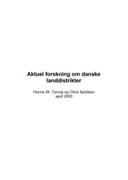
A typical biomass growth function
Biomass
growth,
G i (x)
[x´]
[x´´]
x i

The Community Matrix
(An (I×I)(
I) non-symmetric matrix
of marginal interaction terms)
G
x
( x)
1 1
⎛Gx
. . G ⎞
1
xI
⎜
⎟
2
∂G( x)
⎜ . G
x
. ⎟
∂x
⎜ . . . ⎟
⎜
I
I
Gx
. . G ⎟
⎝ 1
xI
⎠
2
≡ = ⎜ ⎟
i i
Note: G ≡ G ( x),
i.e. the interaction terms, are functions of biomass
x
j
x
j

If the community matrix is diagonal..
Gx
( x)
⎛G
⎜
⎜
1
x
1
0 . 0
2
0 Gx
0 .
2
= ⎜ ⎟
⎜
⎜
⎝
. 0 . 0
0 . 0
G
I
x
I
⎞
⎟
⎟
⎟
⎟
⎠
....then there are no interspecies,
ecological effects

Important things to notice about the
ecosystem equation &x = G( x, z)
1. It may (and probably will) exhibit multiple
equilibria
2. It may easily exhibit complicated
dynamics
(1) Strange attractors
(2) Bifurcations
(3) Chaos

Illustration of multiple equilibria
alpha⋅x
− beta⋅x 2
ay ⋅ − by ⋅
2
4
− cx ⋅ 0
− gamma⋅
y 0
gamma = -1, c = 1
=> x prays on y
Locally
stable
Fxx ( )
Hxx ( )
y
HH( xx)
− 2
0
0 2 4
0 xx
Saddle
point
4

Species interactions creating chaos
- A very simple example -
x − t 1
x = t
a ⋅ x ⋅ + t
(1 − b ⋅ xt)
3
y − 1
y = α ⋅ x ⋅ (1 − +
β ⋅ x ) − γ ⋅ y ⋅ x
t t t t t t
a=1.5 α=2.0
b=0.5 β=0.5
γ = ?

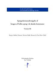
Dynamics
γ = 0
γ = 0.233
2.067
3
2.067
3
2
2
1
1
0.8
x i
200
0
0 100 200
0.8
x i
200
0
0 100 200
1 i
1 i
3
3
3
2
2
1
1
0 50 100
1 i
100
y i
0.039
y i
100
0
0 50 100
1 i

Harvesting Activity
• Harvesting sector consists of
(i)
N harvesting firms (here aggregated)
(ii) Rest of the economy
• Rest of the economy represented by prices
(assumed to be constant => not a GE model)

Fishing effort
Vector of species directed fishing effort
e = (e 1 ,e 2 ,....e I )
• If the e i s can be freely selected, we have
perfect targetting
• If not, e.g. e i = F(e j ) ..etc, we have
limited targetting.

Harvesting function
i
y = Y ( ex , ), i = 1, 2,... I
i
∂Y
∂x
∂Y
∂e
i
j
j
i
≠
≠
0, cross species stock effects
0, by-catch
y
= Yex (, )

Biomass Evolution
&x = G( x, z) −Y( e, x)
i
i
x& = G ( xz , ) −Y ( ex , ), i=1,2,...
I
i

Cost Function
i
c = C ( ew , ), i = 1, 2,... I
i
∂C
∂e
j
i
≠
0, production externality
c=C( e,w)

Profits
i
i
π
i
= Y ( ex , ) − C ( ew , ), i = 1, 2,... I
π = Yex (, ) − Ce,w ( )
I
i
i
π = π = Y (, ) −C
(, )
i
i= 1 i=
1
I
∑ ∑ ex ew
= 1⋅( Yex ( , ) − Cew ( , )) = 1⋅π

Present value of profits
∞
−rt
⋅
−rt
⋅
V = π ⋅ e dt = 1⋅( Yex ( , ) −Cew
( , )) ⋅e dt
∫ ∫
0 0
∞

Optimal Ecosystem Use

Optimal Ecosystem Fisheries
−rt
⋅
−rt
⋅
Max V = π ⋅ e dt = ⋅( Yex ( , ) −Cew
( , )) ⋅e dt
{} e
∞
0 0
∞
∫ ∫ 1
Such that &x = G( x) -Y( e,x)
e ≥ 0
x ≥ 0

Necessary Conditions
(Assuming e, x>0) x
H = λ 0
⋅1⋅( Y( e, x) − C( e, w)) + λ ⋅( G( x) -Y( e,x))
λ
0
= 1
1
e e
⋅Π − λ ⋅Y
=
λ&
−r
⋅ λ=−1⋅Y −λ⋅(
G −Y
0
x x x
)
&x
=
G( x) -Y( e,x)
(3⋅I conditions to determine 3 ⋅I unknowns)

Interpretation
Rule for optimal vector of fishing effort at each
point of time:
⋅Π − λ ⋅Y
= 0
1
e e
Rule for determining the vector of shadow values
of biomass:
λ&
−r
⋅ λ=−1⋅
−λ⋅(
−
Y G Y
x x x
)

Note!
• Single species solutions are appropriate
only if all four (I×I)(
) matrices;
Y e , Y x , C e and G x
are diagonal!
Theorem
Even when there are no ecosystem interactions,
economic interactions (bycatch, cross stock
externalities and production externalities) will
generate similar complexities

Concentrated Solution
λ&
=− 1⋅Y + λ⋅ ( Y + r ⋅I
−G
x x x
),
λ =
1
e e
⋅Π ⋅( Y ) −1
&x
=
G( x) -Y( e,x)
This system of 2⋅I2
differential equations may
exhibit very complex dynamics!
(incl. multiple equilibria, , strange attractors and chaos)

Equilibrium equations
x&
= e&
= 0
λ Π I
1
⋅ [ G ( ) −
x
+ Ce⋅ e
⋅Yx
−r
⋅ ) = 0
λ =
1
e e
⋅Π ⋅( Y ) −1
G( x) -Y( e,x) = 0

Properties of equilibrium
1. There may be many solutions (equilibria(
equilibria)
2. The stability properties of these equilibria may
be of many kinds
3. In the single species case, I=1, the system
reduces to the usual Clark-Munro equilibrium
solution
Ce⋅Yx
Gx ( ) + = r
π
Gx ( ) − Yex ( , ) = 0
e

Properties of equilibrium ...cont.
4. If (and only if) all the Jacobian matrices, Y e , Y x , C e
and G x are diagonal, the equilibrium system
reduces to a collection of Clark-Munro single
species equilibrium expressions.
5. The shadow values of biomass, λs, do not have to
be positive!

Example of equilibrium
Two species
λ Π I
1
⋅ [ G ( ) −
x
+ Ce⋅ e
⋅Yx
−r
⋅ ) = 0
1 1 1 1 1 1
−1
⎛
1 1
⎛Gx G ⎞ ⎛
x
Ce C ⎞ ⎛
e
Πe Π ⎞ ⎛
e
Yx Y ⎞
x 1 0
⎞
⎛ ⎞
⋅ ⎜ + ⋅ ⋅ −r
⋅ ⎟=
1 2 1 2 1 2 1 2
( λ1, λ2) 0
2 2 2 2 2 2 2 2
⎜⎜G 0 1
x
G ⎟ ⎜
1 x
C
2 e
C ⎟ ⎜ ⎟ ⎜ ⎜ ⎟
1 e2 e1 e
Y
2 x
Y ⎟ ⎟
⎝ ⎠ ⎝ ⎠ ⎝
Π Π
⎠ ⎝ 1 x ⎝ ⎠
2 ⎠
⎝
λ
G + Ψ + ( G + Ψ ) ⋅ = r,
λ
1 1 2 2 2
x1 1 x1
1
1
λ
G + Ψ + ( G + Ψ ) ⋅ = r
2 2 1 1 1
x2 2 x2
2
λ
2
⎠
where
⎛
1 1 1 1
−1
1 1
1 1
Ψ Ψ ⎞ Ce Ce Πe Πe Yx Yx
≡ ⋅ ⋅
⎛ ⎞ ⎛ ⎞ ⎛ ⎞
1 ¨2
1 2 1 2 1 2
⎜ 2 2 ⎟
2 2 2 2 2 2
⎝Ψ1 Ψ2
⎠
⎜Ce C ⎟ ⎜ ⎟ ⎜
1 e2 e1 e
Y
2 x
Y ⎟
⎝ ⎠ ⎝
Π Π
⎠ ⎝ 1 x2
⎠

Ecosystem Management

Behaviour
Optimal
1
e e
⋅Π − λ ⋅Y
=
I
I
i i i i
ej ej ∑λ
ej
i= 1 i=
1
∑
( Y −C ) − ⋅ Y = 0, j = 1, 2,... I
0
Common Property
⋅Π =0 1
e
So, the management problem is to
impose the shadow prices, λ i s !

Taxes
Optimal shadow prices:
Define the tax (on harvest):
λ =
τ =
⋅Π ⋅( Y ) −1
1
e e
⋅Π ⋅( Y ) −1
1
e e
Profits become:
1⋅Π(, ex) −τ ⋅Y( e,x)
Behaviour becomes: 1⋅Π − τ ⋅Y
= 1⋅Π − λ⋅Y
= 0
e e e e
Optimal!

Problem
The optimal tax vector depends on e* and x*
τ = Y F x e
parameters
−1
1⋅Πe⋅ (
e) = ( *, *, )
Therefore to calculate the optimal tax, one must
first solve the dynamic optimization problem
This is a hard task indeed!!

An ITQ system
1. Fishing firms hold fractions of the TAC for each
species: Share quotas, α(i,t)
2. The share quotas are permanent assets
3. “Annual” catch quota: q(i,t)= α(i,t)⋅TAC(t)
4. Both types of quotas are divisible and tradable ⇒
(i)
quota holdings can be adjusted over time
(ii) there will be quota prices
5. Fisheries authorities decide on
(i)
initial allocation of share quotas
(ii) total allowable catches “annually” TAC(t)

Quota prices
• Under this ITQ system, the quotas (both catch quotas
and the share quotas) will have a price
• Let s be the price of the catch quota
• Note that s can be negative!
• Now, s represents the opportunity cost of harvest
(just as a tax or a shadow value)
• It follows that behaviour will be:
1
e e
⋅Π − sY ⋅ =
0

Optimal behaviour under ITQs
• If s=λ ⇒ behaviour will be optimal!
• But s depends on the
vector of TACs (the
total allowable catches)!
s
TAC
⇒ By setting the right TACs the quota authority
will induce the optimal fishing behaviour

How to set the right TAC?
• To calculate the right TAC requires solving the
dynamic maximization problem
• Not really feasible
• However, the best knowledge about the conditions
of the fishery and thus the “best” possible TAC
resides within the fishing industry
• This information is revealed in permanent quota
prices!!

I
∑
i=
1
Can show that:
∞
−rt
Si
= 1⋅ S = ∫ 1⋅π
⋅e dt
0
S = Share quota price
Theorem
Permanent quota prices equal
expected present value of profits in
the fisheries

So in order to find the “best” TAC,
the quota authority only has to play
around with the TACs !!

Example for one species
Quota values,
resource
rents
Total allowable catch, TAC

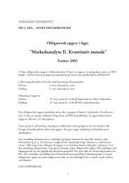
Example for two species
Quota
value
TAC 2
M
TAC 1

Will this work?
1. Needs well functioning quota markets
2. Will not be fully optimal (unless
information is perfect)
3. It will be as good as socially possible, i.e.
it will use (and generate) information
efficiently
[Market arbitrage arguments]

Optimal ecosystem fisheries
(Probable outcome)
Quota price
Total Quota, TAC
Negative
(i.e., stock enhancement)
Positive
(i.e., fishery)
Negative
Positive
Unprofitable stock
enhancement
(subsidized releases)
Profitable stock
enhancement
(ocean ranching)
Unprofitable fishery
(subsidized removal
of predators/competitors)
Profitable fishery
(Commercial fishery)

Summary
1. Ecosystems are exceedingly complex
2. There is virtually no chance that empirical
research will reveal their structure within our
lifetimes
3. It follows that sensible management is very
difficult to achieve
– Akin to groping in the dark
– Decision making under extreme uncertainty and very
high risk.

Summary ....cont.
4. Under these circumstances centralized
management is particularly unattractive
– Inappropriate incentives
– Information collection and processing
5. Decentralized decision making collects and
processes available information much better
– Cf. the market system
6. Ecosystem ITQs greatly facilitate dealing with
this ecosystem uses.

Summary ....cont.
7. Analysis of the workings of ecosystem ITQs
reveals unexpected fisheries management
outcomes
8. Similar approach should apply in natural
resource use in general, .....provided
sufficiently
high quality property rights can be defined and
enforced.
9. This approach does not apply in the case of
environmental public goods.
(In fact, it’s hard to see that market-based approaches
can apply to such to public goods at all)

Strange attractors: Lorenz attractor