A Model of Regulated Open Access Resource Use
A Model of Regulated Open Access Resource Use
A Model of Regulated Open Access Resource Use

Create successful ePaper yourself
Turn your PDF publications into a flip-book with our unique Google optimized e-Paper software.
Ž .<br />
JOURNAL OF ENVIRONMENTAL ECONOMICS AND MANAGEMENT 32, 121 1997<br />
ARTICLE NO. EE960947<br />
A <strong>Model</strong> <strong>of</strong> <strong>Regulated</strong> <strong>Open</strong> <strong>Access</strong> <strong>Resource</strong> <strong>Use</strong>*<br />
FRANCES R. HOMANS<br />
Department <strong>of</strong> Applied Economics, Uniersity <strong>of</strong> Minnesota, St. Paul, Minnesota 55108<br />
AND<br />
JAMES E. WILEN<br />
Department <strong>of</strong> Agricultural and <strong>Resource</strong> Economics, Uniersity <strong>of</strong> California at Dais, Dais,<br />
California 95616, and Giannini Foundation<br />
Received October 5, 1994; revised August 24, 1995<br />
This paper develops a model <strong>of</strong> regulated open access resource exploitation. The regulatory<br />
model assumes that regulators are goal oriented, choosing target harvest levels according<br />
to a safe stock concept. These harvest quotas are implemented by setting season lengths,<br />
conditioned on the industry fishing capacity. The industry enters until rents are dissipated,<br />
conditioned on season length regulations. Harvest levels, fishing capacity, season length, and<br />
biomass are determined jointly. Using parameter estimates from the long-regulated North<br />
Pacific Halibut fishery, predictions <strong>of</strong> these variables from the regulated open access model<br />
are compared to predictions that arise from the Gordon model. 1997 Academic Press<br />
1. INTRODUCTION<br />
A survey <strong>of</strong> the literature in fisheries economics would leave one with the<br />
impression that fisheries fall into one <strong>of</strong> two institutional configurations: pure open<br />
access or optimized rent maximizing. This impression would be conveyed because<br />
these two paradigms totally dominate the published literature in fisheries economics.<br />
At the same time, if one were to examine the institutional configurations<br />
under which real world fisheries operate, one would find virtually no fisheries<br />
operating under either pure open access or rent maximizing conditions. Instead,<br />
most <strong>of</strong> the world’s most important fisheries operate under what might best be<br />
termed regulated open access. In regulated open access fisheries, participants are<br />
free to enter but subject to certain regulations imposed by a management agency.<br />
These typically take the form <strong>of</strong> gear restrictions, area closures, and importantly,<br />
season length restrictions. 1<br />
Economists have not, <strong>of</strong> course, ignored regulations in discussions <strong>of</strong> fisheries.<br />
As early as the fifties, economists were hypothesizing about the economic impacts<br />
<strong>of</strong> regulations on fisheries, including output and input taxes, gear restrictions, and<br />
time and area closures, among others. 2 These somewhat speculative discussions<br />
arose in a particular institutional context in which most <strong>of</strong> the world’s important<br />
* The authors acknowledge helpful comments from three anonymous referees. This is Minnesota<br />
Agricultural Experiment Station Paper 21, 494.<br />
1 Some fisheries also operate under a more stringent form <strong>of</strong> regulation, in which regulations are<br />
imposed and enforced in a restricted access setting that uses a license limitation scheme or another<br />
form <strong>of</strong> closure to entry. These are perhaps best viewed as regulated restricted access fisheries.<br />
2<br />
Cf. Turvey and Wiseman 22 , Scott 18 , and Crutchfield and Zellner 8 .<br />
1<br />
0095-069697 $25.00<br />
Copyright 1997 by Academic Press<br />
All rights <strong>of</strong> reproduction in any form reserved.
2<br />
HOMANS AND WILEN<br />
fisheries were virtually unregulated and operating under open access conditions.<br />
H. S. Gordon’s 10<br />
important paper had just appeared, pointing out how open<br />
access fisheries inevitably dissipate potential rents and as a result, economists’<br />
early discussions about regulations focused on normative issues such as: how can<br />
regulations be designed in order to coax an open access fishery closer to a rent<br />
maximizing ideal? The extension <strong>of</strong> jurisdiction by coastal nations in 1976 changed<br />
the institutional context <strong>of</strong> fisheries dramatically since virtually all <strong>of</strong> the most<br />
important fisheries suddenly came under the authority <strong>of</strong> adjacent coastal nations.<br />
This important change set the stage for a new era <strong>of</strong> regulated fisheries use by<br />
legitimizing coastal nations’ authority to explicitly manage the use <strong>of</strong> their fisheries.<br />
As coastal nations have begun to exert more regulatory control over their<br />
adjacent fisheries, economists have continued to focus primarily on normative<br />
issues associated with regulatory design. There have been several important policy<br />
contributions emerging from this work. Economists were instrumental, for example,<br />
in framing management legislation Ž such as the Magnuson Act.<br />
in a manner<br />
that incorporated socioeconomic as well as biological goals and in promoting<br />
rationalization schemes including limited entry and transferable quota schemes.<br />
Interestingly, however, in their descriptive analytical and empirical work, economists<br />
have continued to depict fisheries as if they are still operating under pure open<br />
access conditions. This is in spite <strong>of</strong> the fact that most modern fisheries are heavily<br />
influenced by regulatory structures which proliferated especially after the extension<br />
<strong>of</strong> coastal jurisdictions at the end <strong>of</strong> the seventies.<br />
A question which might be asked is, why not simply incorporate regulations as<br />
technological constraints and treat them as a minor modification <strong>of</strong> the basic open<br />
access model? The answer to that question is that the regulatory structure is<br />
fundamentally more important than this, particularly as a force affecting the<br />
character <strong>of</strong> fisheries in the long run. Moreover, regulatory constraints are not<br />
simply exogenous but instead are fluid and an outcome <strong>of</strong> purposeful behavior by<br />
institutions with goals and objectives. The menu <strong>of</strong> regulatory instruments is <strong>of</strong>ten<br />
extensive and regulators actively choose both the suite <strong>of</strong> instruments and their<br />
respective levels in a manner that reflects current and expected future conditions<br />
in each fishery. When external factors change, regulations also change in response<br />
and hence regulations are fundamentally endogenous and dynamic.<br />
The implications <strong>of</strong> these observations are at least three. First, the technological<br />
and behavioral character <strong>of</strong> modern fisheries is intimately bound up with the<br />
nature and operation <strong>of</strong> the regulatory structure. Not only will technology and<br />
behavior be affected by the regulatory structure, but so also will the health and<br />
attributes <strong>of</strong> the harvested species. Second, discussions <strong>of</strong> policy alternatives need<br />
to measure the gains from rationalization relative to the appropriate status quo.<br />
<strong>Regulated</strong> fisheries may look considerably different from what would emerge<br />
under pure open access and they may, in fact, even be generating substantial<br />
economic rents. Finally, modeling the evolution <strong>of</strong> fisheries and particularly forecasting<br />
future conditions must account for not only the dynamics <strong>of</strong> the biomass<br />
and the technology and behavior <strong>of</strong> the industry but also the dynamics <strong>of</strong> the<br />
behavior and technology <strong>of</strong> the regulatory apparatus. This places an even greater<br />
burden on modelers to know and understand the particular features <strong>of</strong> the fisheries<br />
they are modeling.<br />
In this paper we present a model <strong>of</strong> a regulated open access fishery which we<br />
believe more accurately captures some <strong>of</strong> the features <strong>of</strong> modern fisheries. It is
REGULATED OPEN ACCESS RESOURCE USE 3<br />
important to highlight that this is a predictive rather than a normative model; we<br />
are interested in modeling and understanding the implications <strong>of</strong> structures which<br />
exist in real world setting rather than addressing questions about whether they are<br />
efficient or which institutions might be optimal. The model developed elevates the<br />
role <strong>of</strong> the regulatory structure to one on par with consideration <strong>of</strong> industry<br />
behavior and biological dynamics. We treat the regulatory sector as rational and<br />
purposeful Ž although not necessarily efficient ., so that regulatory behavior and<br />
industry behavior jointly and endogenously determine the character <strong>of</strong> the fishery<br />
in question. We also view the process <strong>of</strong> regulatorindustry interaction as dynamic<br />
so that when internal and external conditions change, the regulatory sector<br />
responds rather than being considered simply exogenous. In the next section the<br />
conceptual model is discussed and in Section 3 this model is used to generate some<br />
hypotheses about regulated open access fisheries. Section 4 discusses results <strong>of</strong> an<br />
empirical application <strong>of</strong> the model and the concluding section summarizes the<br />
differences between our model <strong>of</strong> regulated open access use and the more widely<br />
used pure open access model.<br />
2. A MODEL OF A REGULATED OPEN ACCESS FISHERY<br />
The model developed here has three fundamental components. First, in the<br />
industry component, it is assumed that the fishing industry commits a given amount<br />
<strong>of</strong> fishing capacity each season, based upon anticipated prices, costs, biomass level,<br />
and Ž importantly.<br />
the regulations set by the regulatory agency. Second, in the<br />
regulatory component, it is assumed that the regulatory agency selects regulations,<br />
based upon specific biologically oriented goals and the anticipated fishing capacity<br />
level <strong>of</strong> the industry. Thus there is a joint equilibrium established between the<br />
industry and the regulatory sector. Finally, in the biological component, we assume<br />
that the biomass evolves between seasons in a manner dependent upon how much<br />
has been harvested each season and the initial biomass level. The fishery is<br />
characterized by an equilibrium consisting <strong>of</strong> fishing capacity and regulation levels<br />
determined endogenously, and the biomass level. 3 The motivation for the specific<br />
characterizations <strong>of</strong> these components are as follows.<br />
2.1. Fishermen’s Behaior<br />
H. S. Gordon’s model <strong>of</strong> rent dissipation is a useful point <strong>of</strong> departure for<br />
considering industry behavior. We assume that fishermen behave as Gordon<br />
suggested, that is, they enter in response to rents and entry proceeds until effort is<br />
earning its opportunity cost. Rents will be assumed to be the difference between<br />
industry revenues and industry costs, defined over a given fishing season. Revenues<br />
are defined as total seasonal harvest multiplied by an exvessel price P per pound.<br />
Assume that there is an instantaneous Schaefer type harvest function defined by<br />
hŽ t. qEXŽ t ., Ž 1.<br />
3<br />
For a more complete exposition <strong>of</strong> this model, see Homans 13 . An earlier attempt to model<br />
regulation in fisheries as endogenous is in Wilen 24 .
4<br />
HOMANS AND WILEN<br />
where h is the harvest rate, q is the catchability parameter, E is a measure <strong>of</strong><br />
fishing capacity or power, and X is the biomass level in period t <strong>of</strong> a given season.<br />
Assume also that the industry commits an amount <strong>of</strong> capacity E each season so<br />
that E can be considered variable between seasons but fixed within a season.<br />
Let the level <strong>of</strong> biomass at the beginning <strong>of</strong> a particular season be designated<br />
X 0. Assume also that within the fishing season, the biomass declines by the fishing<br />
rate so that:<br />
ẊŽ t. qEXŽ t .. Ž 2.<br />
Between fishing seasons we assume that the biomass grows in a density dependent<br />
fashion so that the beginning biomass level in one season is a function <strong>of</strong> the<br />
biomass level in the previous season. Natural mortality during the season is ignored<br />
here for analytical convenience. In Section 2.3 below we discuss the between-season<br />
dynamics. Under these assumptions, total cumulative harvest for the industry<br />
over a season <strong>of</strong> length T will be<br />
HŽ T. X0XŽ T. X0Ž 1e qET ., Ž 3.<br />
which is determined by integrating Ž. 2 over the season length T, assuming that E is<br />
constant and X0<br />
is given.<br />
With respect to costs we assume simple linear costs related to both the level <strong>of</strong><br />
fixed fishing capacity and to the cumulative level <strong>of</strong> variable effort expended over<br />
the season. Consider capacity costs first. We assume fixed costs <strong>of</strong> f per season per<br />
unit <strong>of</strong> capacity E must be incurred to participate in the fishery. These costs may<br />
be assumed to be outfitting, repair, and preparation costs associated with gear, the<br />
opportunity cost associated with the investment, and other implicit rents associated<br />
with other inputs. We also assume that there are variable costs per unit <strong>of</strong><br />
capacity used per unit time associated with the Ž assumed constant.<br />
rate <strong>of</strong> input<br />
use over the season.<br />
With both cost and revenue formulations as described, we may write total<br />
industry rents anticipated for a season <strong>of</strong> length T as:<br />
qET<br />
Rents PX0Ž 1 e . ET fE . Ž 4.<br />
Total revenues are given by the left hand term and are determined by multiplying<br />
total seasonal harvest in Ž. 3 by the exvessel price P. Total costs are given by<br />
integrating Ž ignoring the discount factor.<br />
variable flow costs E over the season<br />
length T and adding fixed capacity costs <strong>of</strong> fE. Setting rents equal to zero yields an<br />
implicit equation for capacity E as a function <strong>of</strong> T, P, X 0, , f, and q. This gives<br />
the rent dissipating level <strong>of</strong> capacity that would be expected to be attracted into a<br />
fishery in a given season. We are thus assuming that capacity enters each season<br />
until rent dissipation occurs.<br />
The implicit equation JŽ E,T. 0 derived by setting rents in Ž 4.<br />
equal to zero<br />
describes industry behavior associated with capacity levels that dissipate rents,<br />
given a season length T. The functional forms used here, while standard practice<br />
and sensible representations <strong>of</strong> production and cost functions, create some analytical<br />
complexities because it is not possible to explicitly isolate the rent dissipating<br />
capacity E as a function <strong>of</strong> the other variables and parameters. The function<br />
EET;X,P,,f,q Ž . may be analyzed by indirect methods and Fig. 1 depicts the<br />
0
REGULATED OPEN ACCESS RESOURCE USE 5<br />
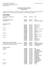
FIG. 1.<br />
Rent dissipating capacity.<br />
shape <strong>of</strong> the function identified by setting Ž. 4 equal to zero Žsee Appendix A for<br />
details ..<br />
The function generally describes a monotonic relationship between E and T<br />
over the relevant range. Other things equal, longer season lengths will require<br />
larger amounts <strong>of</strong> fishing capacity to dissipate rents. Note that there is a minimum<br />
season length Tmin<br />
below which no effort will be attracted, however. This is<br />
because there is a fixed cost f per unit <strong>of</strong> capacity and the season length must be<br />
long enough to generate sufficient variable pr<strong>of</strong>its to cover these costs for the first<br />
unit <strong>of</strong> positive capacity. In addition, there is a maximum capacity Emax<br />
associated<br />
with season length Tmax<br />
which is the longest season length which the industry<br />
would voluntarily choose to use under any circumstance Ž see Appendix A ..<br />
2.2. Regulator Behaior<br />
As discussed in the Introduction, economists have essentially ignored the fact<br />
that regulations are endogenous in modern fisheries. What hypotheses might we<br />
entertain to describe the motivations <strong>of</strong> a regulatory agency? 4 In this paper we<br />
assume a simplified goal structure for the regulatory body which captures the<br />
biological orientation <strong>of</strong> most real world fisheries regulatory bodies. In particular,<br />
we assume a two stage regulatory process where in the first stage, a target harvest<br />
quota is chosen to ensure stock safety. While there are several quota rules which<br />
regulators actually use, a common and analytically simple one is to assume that the<br />
4 One possibility is a rent seeking model, in which constituents are assumed to lobby regulators for<br />
actions that generate rents ŽBhagwati 1 , Buchanan et al. 2 and Rowley et al. 17 . . A related<br />
possibility is a regulatory capture model in which regulatees ‘‘capture’’ the regulators through political<br />
or voting processes and manipulate outcomes ŽKarp<strong>of</strong>f 14 . . These are plausible but at a level in the<br />
policy process once removed from that we are interested in. Fisheries in the United States and<br />
elsewhere are generally managed within broadly defined enabling legislation such as the Magnuson<br />
Fisheries Conservation and Management Act. Fisheries management acts such as this and related laws<br />
specify broad goals for management but not generally how to achieve these goals. Day to day<br />
implementation <strong>of</strong> fisheries regulations is usually left in the hands <strong>of</strong> local, regional, and fishery-familiar<br />
managers housed within biologically oriented field level agencies.
6<br />
HOMANS AND WILEN<br />
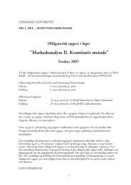
FIG. 2.<br />
Regulator quota rule.<br />
allowable quota or exploitation rate is a linear function <strong>of</strong> the biomass over some<br />
range. 5 The quota would be set, then, according to the rule<br />
Q c dX 0. Ž 5.<br />
In Fig. 2, for example, we show a quadratic yield function with a linear harvest<br />
quota rule superimposed. Whenever the biomass is below the desired long run<br />
‘‘safe’’ stock level, the quota is set below yield so that the biomass grows and<br />
conversely if the biomass is above X safe. This quota rule allows a gradual adjust-<br />
ment toward the equilibrium stock level whenever biomass is above or below it.<br />
Note that if c 0, this rule would also call for a moratorium when the biomass<br />
falls to a level like X , hence a rule like Q maxŽ 0, c dX .<br />
min<br />
better describes<br />
this situation. Note also that this simple rule encompasses the possibility that the<br />
safe stock is the maximum sustainable yield stock as well as others such as the F 0.1<br />
strategy. 6 Obviously other variants <strong>of</strong> these types <strong>of</strong> rules are possible.<br />
In the second stage <strong>of</strong> the regulatory process, we assume that regulatory<br />
instruments are selected to achieve the quota target determined from the quota<br />
rule. This distinction between targets and instruments is important and <strong>of</strong>ten<br />
ignored in descriptive analysis. In real fisheries, it is not enough to simply select an<br />
aggregate harvest level since there is nothing to ensure that the industry won’t<br />
exceed the target. Typical regulatory instruments are the levels <strong>of</strong> various constraints<br />
on fishing technology and practices allowed by regulators, including mesh<br />
size restrictions, area and season length closures, engine size, and gear dimensions.<br />
By far the most commonly used instrument to ensure harvest quota adherence is<br />
the season length restriction. For the model discussed here, we assume that the<br />
5<br />
Cf. the discussion in Hilborn and Walters 12 , p. 2243.<br />
6 The F0.1<br />
strategy prescribes a constant exploitation rate which leaves exploitation slightly less than<br />
the one which maximizes yield per recruit, cf. Hilborn and Walters 12 .
REGULATED OPEN ACCESS RESOURCE USE 7<br />
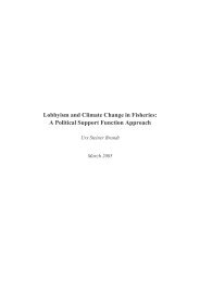
FIG. 3.<br />
Regulator season length choice and joint regulated equilibrium.<br />
relevant instrument is the season length T, although it would be straightforward to<br />
generalize. 7<br />
Suppose that the biomass measured at the beginning <strong>of</strong> the fishing season is X . 0<br />
Then if the quota target is applied to the initial biomass, we have an allowable<br />
harvest quota <strong>of</strong> Q c dX 0, which, if realized, will leave a final end <strong>of</strong> season<br />
biomass <strong>of</strong> X X Ž c dX .. In the second stage, we thus assume that<br />
T 0 0<br />
regulators select the season length instrument level which ensures that the target<br />
will be achieved. This is found by substituting the quota into Eq. Ž. 3 , so that we<br />
have<br />
Q X 1 e qET . 6<br />
0Ž . Ž .<br />
This equation can be solved for the season length T as a function <strong>of</strong> capacity,<br />
beginning biomass, the harvest quota, and the catchability coefficient. In particular,<br />
the regulators are assumed to behave by choosing T so that<br />
1 X 0<br />
T ln . Ž 7.<br />
qE X Q<br />
Note that, once X0<br />
is given, this describes a rectangular hyperbola in T, E space as<br />
shown in Fig. 3. When fishing capacity is large as at point A, regulators will only<br />
allow fishing over a short season but when capacity is low as at point B, a longer<br />
season can be permitted.<br />
A jointly determined regulated open access equilibrium occurs at a capacity level<br />
and season length as depicted at the intersection <strong>of</strong> the two curves. The industry<br />
7 For example, since aggregate fishing capacity is E in our model, we could disaggregate to<br />
incorporate input controls by defining the capacity function to be effective capacity Ž on the grounds.<br />
which is a function <strong>of</strong> various regulatable inputs. If effective capacity is assumed to be a function <strong>of</strong> a<br />
vector <strong>of</strong> inputs, regulators could further be assumed to be able to choose the attributes <strong>of</strong> those inputs<br />
or to regulate their levels directly. For example, fishing capacity is certainly a function <strong>of</strong> gear<br />
dimensions and other specifications and these are almost always directly regulated. The complication<br />
introduced by multiple inputs is that one must also develop a theory about instrument choice which<br />
answers questions like: if both season length and mesh size restrictions can be used to curtail aggregate<br />
effective fishing pressure, how would the mix <strong>of</strong> the two be chosen by regulators?<br />
0
8<br />
HOMANS AND WILEN<br />
equilibrium depicts the industry’s ‘‘choice’’ <strong>of</strong> a rent dissipating capacity, given the<br />
season length, and regulatory behavior is depicted as a choice <strong>of</strong> season length,<br />
given fishing capacity, the initial biomass, and the quota target established in the<br />
first stage.<br />
2.3. Between-Season Dynamics and the Harest Quota Target<br />
The discussions above characterize an industry and regulator equilibrium during<br />
a single fishing season in which the initial biomass and hence quota are predetermined.<br />
If the quota is an equilibrium quota, the biomass will remain constant and<br />
the regulated open access fishery will be in a full steady state. If the biomass is<br />
changing, however, both the industry and regulator equilibrium curves will shift<br />
from season to season, since they are both functions <strong>of</strong> a changing X 0. 8 We can<br />
then think <strong>of</strong> the intersection <strong>of</strong> the two curves as determining a sequence <strong>of</strong><br />
temporary equilibria, in which the industry and regulators attain successive withinseason<br />
equilibria, each associated with the existing biomass level each period. Over<br />
time we would observe the entire system moving through a sequence <strong>of</strong> temporary<br />
seasonal equilibria as the biomass approached its long run level. In order to close<br />
the model and describe this long run equilibrium, we thus need to specify the<br />
dynamic relationships which determine the evolution <strong>of</strong> biomass levels between<br />
seasons.<br />
The simplest way to specify this process is to utilize a hybrid Schaefer<br />
Beverton-Holt model in which within season dynamics are simply governed by Eqs.<br />
Ž. 1 and Ž. 2 above and between season dynamics are governed by a density<br />
dependent mechanism. That is, during the fishing season, total biomass is assumed<br />
to evolve to reflect the harvest rate, falling from its initial level X0 to XT<br />
by the<br />
end <strong>of</strong> the season. Then, between seasons, it is assumed that the net biological<br />
growth depends in some density dependent way on previous biomass. Let X 0, t1<br />
be the biomass at the opening date <strong>of</strong> next year’s season and let XT , t and X0, t be<br />
the ending and beginning biomass levels this season, respectively. Here we are<br />
indexing seasons by t and denoting the beginning and ending dates <strong>of</strong> any<br />
particular season with 0 and T.<br />
Ž .<br />
2 9<br />
Assume that additions to the biomass can be defined as G X0, t aX0, t bX 0, t.<br />
Then between season dynamics can be represented by<br />
X0, t1 XT, t GŽ X0, t. XT, taX0, t bX0, 2 t. Ž 8.<br />
8 In particular, the industry equilibrium function shifts up with increases in biomass. The regulatory<br />
equilibrium function may shift in or out, depending upon the form <strong>of</strong> the quota rule. It can be shown<br />
that the regulatory equation will shift out Ž in. if the regulatory rule is elastic Ž inelastic.<br />
with respect to<br />
biomass. Thus for a linear rule, the rectangular hyperbola will shift out as biomass increases if c is<br />
positive and in if c is negative.<br />
9 Our use <strong>of</strong> the biomass growth function deserves some comment. Since halibut reach reproductive<br />
age in 7 to 8 years, it would be more realistic to employ an age-structured cohort model to capture<br />
biomass dynamics rather than a simple annual model. While the introduction <strong>of</strong> a cohort model may<br />
improve the accuracy <strong>of</strong> our representation <strong>of</strong> biomass dynamics and would be tractable for that<br />
purpose, it would introduce considerable analytical complexities into the complete model <strong>of</strong> season<br />
length and effort determination. Using a lumped parameter annual model for halibut has several<br />
precedents, see Cook 4 , Stollery 21 , and Conklin and Kolberg 5 .
REGULATED OPEN ACCESS RESOURCE USE 9<br />
That is, beginning biomass next season is equal to ending biomass this season plus<br />
net growth added to reproductive activities taking place or near the beginning <strong>of</strong><br />
this season. 10<br />
With between season dynamics operating, under a linear exploitation rate rule,<br />
regulators allow a certain fraction c dX0<br />
<strong>of</strong> the initial biomass to be taken each<br />
season. Thus the harvest target during any season t will be Qt<br />
c dX0, t and we<br />
know that the end <strong>of</strong> the season biomass level will be X X Ž c dX .<br />
T , t 0, t 0, t .<br />
As Fig. 2 shows, a linear exploitation rate leads the biomass to a long run<br />
equilibrium level X safe. When the biomass is below X safe, the linear rule results in a<br />
harvest level below the biological growth and the biomass approaches Xsafe<br />
and<br />
similarly when the biomass is above X safe. Along any path to a steady state,<br />
biomass dynamics may be expressed in terms <strong>of</strong> initial biomass levels, biological<br />
parameters a and b, and the exploitation rate parameters c and d, or<br />
Ž . Ž .<br />
2<br />
X0, t1 1d X0, tc aX0, t bX 0, t. 9<br />
In a long run steady state equilibrium we have<br />
Ž . Ž .<br />
2<br />
X0, t1 X0, t 0 1 d X0, t c aX0, t bX0, t X 0, t, 10<br />
and if we let Xsafe<br />
be the equilibrium value <strong>of</strong> the beginning <strong>of</strong> season biomass, we<br />
have, by substituting into Ž 10.<br />
and solving, the expression<br />
'<br />
2<br />
a d Ž a d.<br />
4bc<br />
Xsafe<br />
. Ž 11.<br />
2b<br />
As expected, this is quadratic, representing the two intersections <strong>of</strong> the quota rule<br />
with the yield curve depicted in Fig. 2. We will assume Ž a d.<br />
is positive and that<br />
the desired steady state is the larger <strong>of</strong> the two roots, which would be considered<br />
the least vulnerable <strong>of</strong> the two stock levels.<br />
Note that since the equilibrium biomass is a function <strong>of</strong> the regulatory parameters<br />
c and d, the notion <strong>of</strong> a safe biomass level is equivalent to a choice <strong>of</strong> the<br />
exploitation rule parameters c and d in the steady state. That is, we can view the<br />
regulatory goal as ensuring that a certain minimal long run biomass is maintained<br />
in the steady state, or alternatively, that the exploitation rule associated with the<br />
parameters is the one which achieves this goal.<br />
10 Alternatively, we could assume that biomass dynamics are governed by the alternative relationship<br />
X X FŽ X .<br />
0, t1 T , t T, t . This formulation would be appropriate if reproductive activities took place<br />
after the fishing season, while X X GŽ X .<br />
0, t1 T , t 0, t would reflect reproduction just prior to the<br />
season opening. The alternative relationship would change the corresponding expression for biomass to<br />
Ž 1a2bc.Ž 1 d. 1 'Ž 1 a 2bc.Ž 1 d. 1 2 4bcŽ 1 d. 2<br />
Ž 1 a bc.<br />
Xsafe .<br />
2<br />
2bŽ 1 d.<br />
Other expressions that embed biomass would change accordingly. Since halibut reproduce in the winter,<br />
just prior to the spring fishing season, the formulation used in the paper reflects halibut biomass<br />
dynamics more accurately than the alternative.
10<br />
HOMANS AND WILEN<br />
3. ANALYSIS OF REGULATED OPEN ACCESS BEHAVIOR<br />
The three components described above characterize a regulated open access<br />
fishery. The industry is assumed to commit capacity E each season until rents are<br />
dissipated. Regulators are assumed to set a harvest target quota Q each season and<br />
then choose a season length T which ensures that the quota is achieved. A<br />
regulated open access equilibrium is achieved by the interaction <strong>of</strong> the industry<br />
and regulators each season. Biomass evolves between seasons according to whether<br />
the corresponding harvest is greater than, equal to, or less than biological growth.<br />
A long run steady state is achieved when the biomass is in equilibrium and when<br />
industry and regulatory behavior are constant.<br />
In a steady state equilibrium, both beginning and ending biomass levels are given<br />
and constant from season and their levels depend upon c, d, a, and b. Since the<br />
harvest quota target is simply the difference between beginning and ending<br />
biomass levels, Q is predetermined also once c and d are chosen. Then a regulated<br />
open access equilibrium within the season is achieved when the industry commits a<br />
level <strong>of</strong> capacity E and the regulators choose a season length T such that<br />
PX0Ž 1 e qET . ET fE 0<br />
1 X0 1 X0<br />
T ln ln , Ž 12.<br />
qE X qE Ž 1 d.<br />
X c<br />
T 0<br />
where X satisfies Ž 11.<br />
0<br />
above. A regulated open access fishery is thus the joint<br />
outcome <strong>of</strong> the behavior <strong>of</strong> both the industry and regulatory agency, coupled with<br />
biological dynamics.<br />
What happens to this equilibrium as economic, regulatory, and biological parameters<br />
change? This can be addressed by performing comparative statics computations<br />
on the equilibrium. Note first that this system is recursive in that the steady<br />
state biomass level is determined only by the biological parameters, a and b, and<br />
the regulatory parameters, c and d. The regulatory agency’s instrument choice T<br />
depends only upon the exploitation rule parameters and the level <strong>of</strong> capacity<br />
chosen by the industry. Thus the two equations in Ž 12.<br />
determine the equilibrium<br />
pair E, T which satisfy the open access regulatory equilibrium. For any arbitrary<br />
X , this pair <strong>of</strong> equations yields a temporary equilibrium ET,X Ž .,TŽ E, X .<br />
0 0 0<br />
dependent upon X , and when X satisfies Ž 11 .<br />
0 0<br />
, the system is in a full long run<br />
equilibrium with X0<br />
constant.<br />
Comparative statics properties <strong>of</strong> the long run equilibrium are given in Table I<br />
and Appendix B. These are all plausible results. When prices P or harvest<br />
efficiency q rise Ž or costs or f fall.<br />
the rent dissipating level <strong>of</strong> E rises. But if the<br />
biomass and quota are in long run equilibrium, this increase in potential fishing<br />
capacity must be stifled by corresponding reductions in season length. Since the<br />
biological system is recursive, pricecost parameters do not affect the steady state<br />
level <strong>of</strong> biomass which is determined only by biological and regulatory parameters<br />
Ž a, b, c, and d .. On the other hand, changes in a, b, c, and d affect the levels T<br />
and E in potentially complicated ways via their effects on X and Q. For example,<br />
if the intrinsic growth rate a rises, then Žceteris paribus; holding the exploitation<br />
rule constant.<br />
both the allowable long run biomass and quota will rise. As it turns
REGULATED OPEN ACCESS RESOURCE USE 11<br />
TABLE I<br />
Comparative Statics<br />
Variable<br />
E T X Q<br />
P 0 0<br />
0 0<br />
f 0 0<br />
q 0 0<br />
a <br />
b <br />
c ? ? ?<br />
d ? ? ?<br />
out, this higher quota is achieved with an increase in the equilibrium level <strong>of</strong><br />
fishing capacity and a decrease in the regulated season length.<br />
The only ambiguous results are those associated with the effects <strong>of</strong> changes in<br />
the regulatory parameters c and d on E and T. Recall that increasing the quota<br />
rule parameter d reduces the steady state biomass level while it increases the<br />
fraction <strong>of</strong> initial biomass targeted for harvest. Thus whether or not an increase in<br />
d will attract more entry depends upon the interplay between two forces in their<br />
effects on revenues. On the one hand, a lower steady state biomass level will<br />
reduce E ceteris paribus because there is a stock effect via the production function.<br />
On the other hand, increasing the exploitation rate increases the fraction <strong>of</strong> initial<br />
biomass allowed to be taken. If d is such that the steady state biomass is to the<br />
right <strong>of</strong> X msy, then increasing d has opposing effects: a reduction in revenues via<br />
the stock effect <strong>of</strong> a reduced biomass level on the harvest function, and an increase<br />
in revenues via the fact that lower biomass levels actually increase the amount <strong>of</strong><br />
growth and hence steady state yield. If d is relatively large, however, so that the<br />
equilibrium is to the left <strong>of</strong> X msy, increases in d cause a negative stock effect and a<br />
reduction in allowable harvest, both <strong>of</strong> which lead to lower E and longer T. The<br />
bottom line is that for large enough values <strong>of</strong> d, the derivative <strong>of</strong> E with respect to<br />
d is negative and the derivative <strong>of</strong> T with respect to d is positive, whereas for<br />
smaller values these signs are indeterminate.<br />
Note that the qualitative properties <strong>of</strong> the regulated open access model are<br />
different from those predicted by the pure open access Gordon model in fundamental<br />
ways. In the Gordon model, rents generate excess capacity, which in turn<br />
results in excessive harvest levels. These harvest levels, coupled with biological<br />
dynamics, determine an approach to a bioeconomic equilibrium. With higher prices<br />
andor lower costs, the bioeconomic equilibrium will occur at lower, more vulnerable<br />
biomass levels. In the model presented here, the existence <strong>of</strong> the regulatory<br />
structure decouples the effects <strong>of</strong> economic parameters from impacts on the<br />
biomass. To the extent that the regulatory structure is effective, the biomass level<br />
will approach its safe level. Harvest quota targets ensure this, but the manner in<br />
which they are implemented depends upon the interplay between biological and<br />
economic factors. For example, when prices are high, potential rents attract more<br />
capacity which is stifled on the grounds with short seasons so that the targeted<br />
harvest quota is not exceeded. In the long run the regulated open access fishery
12<br />
HOMANS AND WILEN<br />
will be characterized by higher biomass levels and generally even higher levels <strong>of</strong><br />
inefficient input use than the Gordon model would predict.<br />
4. AN APPLICATION THE NORTH PACIFIC HALIBUT FISHERY<br />
The North Pacific Halibut fishery provides a good case study with which to<br />
estimate and test some <strong>of</strong> the hypotheses generated from the model <strong>of</strong> regulated<br />
open access described above. In the first place, the fishery has a long history <strong>of</strong><br />
regulation dating back to the 1930s. Over this whole period, an extensive data<br />
collection effort has been maintained in order to regulate the fishery. Long time<br />
series exist on measures <strong>of</strong> fishing capacity, total fishing effort expended, biomass<br />
estimates, quota targets, season lengths, and other economic variables. Second, the<br />
halibut fishery has been conducted with relatively simple fishing technology over<br />
the whole period, a longline gear with fairly standardized design and under<br />
relatively constant practices. Third, the halibut fishery has been managed over this<br />
whole period under a structure much like that described above. In particular,<br />
harvest quotas have been set by regulators annually and season lengths have been<br />
used to constrain the application <strong>of</strong> fishing pressure in order to achieve the desired<br />
harvest target.<br />
We assembled data from sources published by the International Pacific Halibut<br />
Commission Ž IPHC.<br />
over the 19351977 period. Two separate series were constructed<br />
as a consistency check <strong>of</strong> the models, one for each <strong>of</strong> two management<br />
areas referred to as Area 2 Ž<strong>of</strong>f British Columbia and up to Cape Spencer in<br />
Southeastern Alaska.<br />
and Area 3 north <strong>of</strong> Cape Spencer <strong>of</strong>f Alaska but excluding<br />
waters in the Western Aleutians and Bering Sea ..<br />
11 The data used include biomass<br />
estimates from Quinn et al. 16<br />
which were computed from logbook entries over<br />
the entire halibut program history. These are computed ex post, <strong>of</strong> course, but we<br />
assume they are unbiased representations <strong>of</strong> estimates used by regulators over the<br />
period for seasonal regulation decisions, as well as by the industry for capacity<br />
commitment decisions. Our measure <strong>of</strong> fishing capacity is also derived from<br />
logbook information. These data were used to calculate the total number <strong>of</strong><br />
standard skate soaks Žunits <strong>of</strong> longline gear, approximately 1800 feet long with 100<br />
hooks attached at 18 foot intervals, set in the water for 12 hours.<br />
in each area,<br />
which we divided by season length to estimate average fishing capacity. This<br />
measure thus assumes that effort intensity does not vary over the sample and that<br />
each unit <strong>of</strong> standardized capacity has costs proportional by their conversion<br />
factors to actual costs. Harvest and price data are also derived from published<br />
IPHC sources and prices are deflated by a wholesale price index with base year<br />
1982. Quotas for each <strong>of</strong> the areas are published in annual reports by the IPHC.<br />
Season lengths were derived from published annual reports by the IPHC and from<br />
a summary in Skud 20 . These are expressed in days <strong>of</strong> season length and are<br />
essentially continuous over the period examined.<br />
11 The period <strong>of</strong> estimation was truncated at 1977 for several reasons. First, the jurisdiction extension<br />
by both Canada and the U.S. led to a separation <strong>of</strong> the waters <strong>of</strong> Area 2 into separate Canadian and<br />
U.S. waters, each with new data collection procedures and management methods. In addition, Canada<br />
instituted a limited entry program in 1979 which would have added estimation complications associated<br />
with expected change in industry and perhaps regulatory behavior.
REGULATED OPEN ACCESS RESOURCE USE 13<br />
The econometric model consists <strong>of</strong> four structural equations: the biomass growth<br />
function Ž. 8 , the quota rule Ž. 5 , the entryexit equation Ž. 4 , and the season length<br />
determination function Ž. 7 . Econometric error terms are appended to each <strong>of</strong> these<br />
equations, so that the model becomes<br />
Xt Ht1 Ž 1 a. Xt1bXt1 2 1t<br />
Ž 13.<br />
QtcdXt 2t<br />
Ž 14.<br />
1 X t<br />
Tt ln 3t<br />
Ž 15.<br />
qE X Q<br />
t t t<br />
qE<br />
<br />
t T<br />
0PX 1e t<br />
ET fE f E D . Ž 16.<br />
t t t t t w t WAR 4t<br />
Since the biomass level is predetermined each year, and the quota is set based<br />
upon the predetermined biomass level, Eqs. Ž 13. and Ž 14.<br />
are estimated individually<br />
using ordinary least-squares. The capacity level and the season length are<br />
determined simultaneously in equations Ž 15. and Ž 16.<br />
once the biomass and quota<br />
are known. We allow for a nonzero covariance between 3t<br />
and 4 t and impose the<br />
cross equation restriction that the catchability coefficient q is the same in both<br />
equations. Because <strong>of</strong> the simultaneity, the correlation in the error terms, and the<br />
cross-equation restriction, Eqs. Ž 15. and Ž 16.<br />
are estimated jointly using nonlinear<br />
three-stage least-squares. All the predetermined variables in the system Ž P, Q, X,<br />
and D . as well as the regulatory variable ŽlnXŽ X Q..<br />
WAR<br />
and lagged values<br />
for E, T, and X were used as instruments.<br />
The entryexit equation Ž 16.<br />
is modified slightly by including a dummy variable<br />
for the war years. Since our estimation period spans the disruptive World War II<br />
years, we modify the fixed cost coefficient by including a dummy variable Ž D WAR<br />
.<br />
for the years 19431945 when the war was active in the Pacific. Management<br />
reports suggest that fishermen were explicitly warned against fishing in the Bering<br />
Sea during the war due to dangers posed by Japanese submarines.<br />
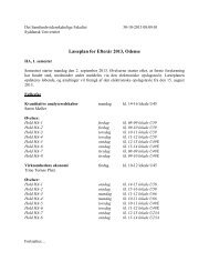
Results are presented in Table II. The biological dynamics and quota rule results<br />
are also shown in Fig. 4. The quota rule equation was corrected for autocorrelation,<br />
while the biological growth function was not. 12 The parameter estimates for<br />
these equations are all reasonable: the signs are as expected and all coefficients are<br />
significant at the 5% level, with most significant at the 1% level.<br />
The implies maximum biomass levels are 318 and 416 million pounds for Areas 2<br />
and 3, respectively. Maximum sustainable physical yields occur at half <strong>of</strong> these<br />
12<br />
Durbin’s h tests indicate that autocorrelation is present in equation Ž 13 .. Our suspicion is that the<br />
positive test for autocorrelation, along with the recognition that the age <strong>of</strong> recruitment is 78 years, is<br />
an indication that a more complicated lag structure is in order. However, since our principal aim was to<br />
focus on the model <strong>of</strong> regulatory and effort choice rather than on biomass dynamics, we chose to keep<br />
our estimation Ž and our theoretical model.<br />
simple. Among population biologists who have paid serious<br />
attention to these modelingestimation issues Žsee, for instance, Ludwig and Walters 15 . , consensus<br />
seems to be that more accurate representations <strong>of</strong> biological dynamics do not necessarily lead to more<br />
accurate estimates <strong>of</strong> variables <strong>of</strong> interest such as optimum fishing effort or surplus yield. For example,<br />
simple autoregressive specifications <strong>of</strong>ten provide more accurate predictions <strong>of</strong> catch than more<br />
complicated age structured models, which demand more information out <strong>of</strong> limited data sets. Our<br />
corrections for higher order autocorrelation did not change parameter estimates appreciably, indicating<br />
bias associated with autocorrelation in the presence <strong>of</strong> a simple lagged dependent variable on the<br />
right-hand side is not too severe. Our estimates for the yield equations are also in accord with results<br />
from other studies, including Criddle 6 , Criddle and Havenner 7 , Deriso 9 , and Capalbo 3 .
14<br />
HOMANS AND WILEN<br />
TABLE II<br />
Parameter Estimates<br />
Ž .<br />
a<br />
Ž .<br />
a<br />
Ž . Ž .<br />
b<br />
Eq. 13 Eq. 14 Eqs. 16 and 15<br />
Parameter Area 2 Area 3 Area 2 Area 3 Area 2 Area 3<br />
c<br />
c<br />
1a 1.3786 1.3119 <br />
Ž 24.01. Ž 31.51.<br />
b<br />
c<br />
0.00119<br />
c<br />
0.00075 <br />
Ž 2.472. Ž 3.212.<br />
c <br />
c<br />
12.329<br />
c<br />
16.417 <br />
Ž 2.990. Ž 2.807.<br />
d <br />
c<br />
0.0897<br />
d<br />
0.0575 <br />
Ž 2.943. Ž 1.703.<br />
q <br />
c<br />
0.00114<br />
c<br />
0.000975<br />
Ž 24.984. Ž 30.895.<br />
<br />
c<br />
0.0555<br />
c<br />
0.07848<br />
Ž 8.4263. Ž 6.9705.<br />
f <br />
d<br />
1.0318 2.0993<br />
Ž 2.5569. Ž 1.8104.<br />
fW<br />
0.79697 9.6556 d<br />
Ž 1.2154. Ž 3.4284.<br />
0.96 0.92 <br />
Durbin’s h 6.21 5.76 <br />
D.W. 1.33 2.01 <br />
2<br />
R 0.95 0.97 0.94 0.84 <br />
Hansen’s J 1.33 1.49<br />
method OLS OLS NL3SLS<br />
a t-statistics in parentheses.<br />
b Asymptotic t-statistics in parentheses.<br />
c Significant at the 1% level.<br />
d Significant at the 5% level.<br />
biomass levels and the implied levels are 159 and 208 million pounds. The four<br />
parameter estimates can also be used to compute the safe biomass level implied by<br />
regulators’ choices <strong>of</strong> quota levels over this period. Using Eq. Ž 11.<br />
above, the levels<br />
<strong>of</strong> Xsafe<br />
implied by actual choices <strong>of</strong> harvest quota levels over the 19351977<br />
period are 187 and 252 million pounds, respectively. Interestingly, the targeted or<br />
safe biomass levels implied by these equations are greater than the maximum<br />
sustainable yield biomass levels in both Areas 2 and 3, implying a conservative<br />
concern for stock safety.<br />
Results from the estimation <strong>of</strong> the industryregulator behavioral equations are<br />
also given in Table II. Parameter estimates are all <strong>of</strong> the correct sign and generally<br />
significant. Hansen’s J test <strong>of</strong> overidentifying restrictions 11<br />
indicates that the<br />
model is not misspecified. 13 With respect to magnitudes, the parameter estimates<br />
are also reasonable and similar across regions. We would expect higher costs in<br />
13 Hansen’s test is for estimators in the class <strong>of</strong> Generalized Method <strong>of</strong> Moments estimators, <strong>of</strong><br />
which non-linear three stage least-squares is one. It is calculated as the value <strong>of</strong> the criterion function<br />
multiplied by the number <strong>of</strong> observations, and has a Chi-square distribution where the degrees <strong>of</strong><br />
freedom are the number <strong>of</strong> instruments Ž. 8 less the number <strong>of</strong> free parameters Ž. 4 . Since Eq. Ž 16.<br />
is an<br />
implicit equation where the dependent variable is zero, there is no adequate goodness <strong>of</strong> fit measure<br />
available.
REGULATED OPEN ACCESS RESOURCE USE 15<br />
FIG. 4.<br />
Quota rule targets.<br />
Area 3 due to its remoteness and this is the case for fixed costs. Fixed cost<br />
estimates suggest a tw<strong>of</strong>old difference, with gear up cost estimates about $1,030 per<br />
unit <strong>of</strong> gear in Area 2 and $2,100 in Area 3. The War also had the expected effect<br />
<strong>of</strong> increasing the implicit opportunity cost <strong>of</strong> participating in the fishery. The<br />
implicit opportunity costs added by the hazards <strong>of</strong> war amount to an extra $790 per<br />
unit <strong>of</strong> gear in Area 2 and almost $9,700 in the Bering Sea. Variable costs are<br />
about $56 and $78 per gear set Ž skate soak.<br />
in Areas 2 and 3, respectively. This<br />
suggests that operating costs are lower in the more accessible region.<br />
5. IMPLICATIONS AND ANALYSIS<br />
The predictions generated from this model <strong>of</strong> regulated open access are significantly<br />
different from those from the standard open access paradigm. In view <strong>of</strong> the<br />
fact that most fisheries are regulated rather than pure open access, we should also<br />
expect that they are closer to what we observe in real fisheries. In this section we<br />
compare the predictions <strong>of</strong> our new model with those that would be generated<br />
using the basic H. S. Gordon model <strong>of</strong> open access equilibrium. The issue to be<br />
examined is: what are the implications <strong>of</strong> Ž correctly, we would argue.<br />
including the<br />
regulatory sector in a model <strong>of</strong> a fishery? To examine this question we calculate<br />
the steady state for two alternatives, using parameter estimates described above.<br />
As discussed in the Introduction, the dominant paradigm in the renewable<br />
resource literature is the Gordon model <strong>of</strong> pure open access. We take this model<br />
to be represented by a zero rent condition together with a biological dynamics<br />
equation which describes how the species evolves. We thus assume instantaneous<br />
rent dissipation or fast dynamics for the entryexit <strong>of</strong> fishing capacity, and slow<br />
dynamics for the biology. Since we have also brought into the analysis the concept<br />
<strong>of</strong> a season length, a question arises as to what to assume about TŽ.<br />
t . We assume<br />
that the industry ends up fishing for a period equal to T max, which is the rent<br />
dissipating season length also. In Fig. 1, the industry reaches a temporary equilib-
16<br />
HOMANS AND WILEN<br />
rium which depends upon the biomass level each year, in which Et Ž. Emax<br />
and<br />
TŽ.<br />
t T max. Then, depending upon the corresponding level <strong>of</strong> harvest, the biomass<br />
will either rise or fall in an approach to the open access equilibrium.<br />
The Gordon open access model thus consists <strong>of</strong> three equations<br />
qEŽt.TŽt.<br />
PŽ t. XŽ t. 1e EŽ t. TŽ t. fEŽ t.<br />
0<br />
XŽ t1. Ž 1a. XŽ t. bX Ž t. XŽ t.<br />
1e<br />
2 qEŽt.TŽt.<br />
1 PqXŽ t.<br />
TŽ t.<br />
Tmax<br />
ln<br />
qEŽ t.<br />
<br />
in three unknowns Ž E, T, X .. In the long run steady state, XŽ t.<br />
is constant and the<br />
system is in a full open access equilibrium.<br />
The regulated open access model also includes the rent dissipation equation and<br />
the biological dynamics equation as in the Gordon model above. The principal<br />
difference is that the season length is fixed by regulators in the second stage <strong>of</strong> the<br />
regulatory process, at a length dictated by a quota rule tied to the biomass level.<br />
Thus the regulated open access model consists <strong>of</strong> four equations<br />
qEŽt.TŽt.<br />
PŽ t. XŽ t. 1e EŽ t. TŽ t. fEŽ t.<br />
0<br />
XŽ t1. Ž 1a. XŽ t. bX Ž t. XŽ t.<br />
1e<br />
1 XŽ t.<br />
TŽ t.<br />
ln<br />
qEŽ t. X Ž t. QŽ t.<br />
QŽ t. cdX Ž t.<br />
2 qEŽt.TŽt.<br />
Ž .<br />
which determine four unknowns E, T, X, Q .<br />
We simulated these two systems using parameter estimates from Table II. We<br />
fixed the value <strong>of</strong> the exvessel price at its value in 1977. Table III shows the<br />
equilibrium values predicted by the alternative models for each <strong>of</strong> Areas 2 and 3.<br />
The main differences in predictions from the two models are significant. The<br />
regulated model predicts higher biomass and harvest levels, a higher level <strong>of</strong><br />
capacity and a shorter fishing season. The reason for these differences are, <strong>of</strong><br />
course, associated with the explicit inclusion <strong>of</strong> the regulatory sector. To the extent<br />
that regulations are successful, they hold the biomass at larger levels, which ceteris<br />
paribus generate higher rents and larger levels <strong>of</strong> capacity, which in turn must be<br />
<br />
<br />
TABLE III<br />
<strong>Regulated</strong> vs Unregulated <strong>Open</strong> <strong>Access</strong>: Steady State Predictions<br />
Area 2 Area 3<br />
Gordon <strong>Regulated</strong> open Gordon <strong>Regulated</strong> open<br />
model access model model access model<br />
Capacity 4.5 45.9 2.1 23.6<br />
Season length 79.6 3.3 153.1 5.7<br />
Biomass 37.7 183 56.8 253<br />
Quotayield 12.6 28.7 15.3 30.9
REGULATED OPEN ACCESS RESOURCE USE 17<br />
stifled in order to hold the harvest at the targeted quota. For example, in Area 2<br />
the regulated open access equilibrium has ten times the capacity <strong>of</strong> the unregulated<br />
open access equilibrium. However, instead <strong>of</strong> fishing over 80 days as in the<br />
unregulated case, the regulated season length is only 3 days. The actual values<br />
predicted by the regulated open access model are also relatively close to what has<br />
been observed in the actual fishery recently. For example, total exploitable biomass<br />
in Areas 2 and 3 combined reached about 275 million pounds in the late 1980s.<br />
Area 2 and 3 total harvest levels during the same period averaged about 24 and 55<br />
million pounds, respectively. Season lengths <strong>of</strong>f Alaska in both Areas 2 and 3 have<br />
fallen to about 35 days. 14<br />
The predictions from the regulated open access model point to and explain<br />
several interesting facts about modern fisheries. First, regulated fisheries are likely<br />
to attract even more redundant capital than was predicted by Gordon’s unregulated<br />
open access model. The degree to which this is true depends, in fact, directly<br />
on the degree to which regulations are successful in holding biomass close to a safe<br />
level. At higher biomass levels, more potential rents exist, generating more entry<br />
pressure which must be controlled with efficiency decreasing policies. Second, as<br />
real prices rise Ž due to population growth ., the industry equilibrium curve in Fig. 3<br />
shifts upward, causing the equilibrium to slide along the regulatory equilibrium<br />
hyperbola. Thus it is almost inevitable that over the long run, more capacity is<br />
attracted and regulations are tightened. This explains the process we observe<br />
whereby in many fisheries, seasons have been reduced to a few weeks, days, and<br />
even hours. Finally, this model suggests some important but sometimes counterintuitive<br />
links between regulations, the output market, and rent dissipation. In<br />
particular, as seasons and other regulations are tightened, a likely market consequence<br />
is that exvessel prices are lower than they would otherwise be. For example,<br />
short seasons result in poorly delivered and handled product, and high storage<br />
costs. As prices are affected by regulatory actions, rent dissipating pressures are<br />
actually mitigated somewhat. Thus the direct effects <strong>of</strong> the regulatory process are<br />
to draw in more capacity than the Gordon model would suggest, but dampened<br />
somewhat due to indirect effects <strong>of</strong> regulations on the market. This in turn explains<br />
recent observations about fisheries that have become rationalized with individual<br />
transferable quota Ž ITQ.<br />
programs. In many <strong>of</strong> these, a surprising outcome has<br />
been that most <strong>of</strong> the immediate rent gains have seemed to emerge on the revenue<br />
rather than the cost side. 15 But this is what we would expect: as the system is<br />
released from its restrictive regulatory structure which reduces revenues, the first<br />
easy gains come from new marketing opportunities engendered both the unconstrained<br />
system and also by the new incentives generated under property rights<br />
based regulations.<br />
Rent Dissipating Capacity Function<br />
APPENDIX A<br />
This appendix discusses the shape <strong>of</strong> the equation depicting industry equilibrium<br />
in a regulated open access setting. Industry behavior is assumed to be driven by<br />
14<br />
Cf. U.S. Department <strong>of</strong> Commerce 23 .<br />
15<br />
Cf. Wilen and Homans 25 , Wilen and Homans 26 .
18<br />
HOMANS AND WILEN<br />
rent dissipation in a manner similar to that first described by Gordon in 1954. In<br />
particular, with a Schaefer production function and with biomass dynamics within<br />
the season governed by harvesting mortality, undiscounted rents for any season are<br />
simply<br />
Rents PX0Ž 1 e qET . ET fE. Ž A1.<br />
This equation cannot be solved explicitly for capacity E as a function <strong>of</strong> other<br />
variables. Let JŽ E,T; X , P, q,, f.<br />
0<br />
describe the function obtained by setting rents<br />
in Ž A1.<br />
above equal to zero. Then we can use the implicit function theorem to get<br />
dE JT E PqX0<br />
E qET<br />
. Ž A2<br />
qET<br />
.<br />
dT J T PqX e f<br />
E 0<br />
The denominator <strong>of</strong> this expression is the net value <strong>of</strong> marginal physical product <strong>of</strong><br />
an additional unit <strong>of</strong> capacity. If capacity enters until rents are dissipated, the net<br />
value <strong>of</strong> average physical product will be zero. Since marginal product is less than<br />
average product, and since average product is zero, the denominator must be<br />
negative.<br />
The numerator <strong>of</strong> Ž A2. is the Ž negative <strong>of</strong> the.<br />
value <strong>of</strong> marginal physical product<br />
<strong>of</strong> an additional unit <strong>of</strong> season length. The sign <strong>of</strong> the numerator depends upon<br />
where in the domain <strong>of</strong> ET Ž . we are operating. As it turns out, in the relevant<br />
region, the value <strong>of</strong> marginal product is positive and hence the numerator is<br />
negative. This can be seen as follows. Let Ž ET . be variable pr<strong>of</strong>its associated<br />
with arbitrary levels <strong>of</strong> ET before fixed costs fE are subtracted, or<br />
PX 1 e qET ET. A3<br />
0Ž . Ž .<br />
Note first that is strictly concave in E, T, and ET. In addition, the average<br />
variable pr<strong>of</strong>it function has a finite limit as E approaches zero, namely<br />
This leads to:<br />
lim Ž E. PqX T T . Ž A4.<br />
E0<br />
PROPOSITION 1. A necessary and sufficient condition for positie leels <strong>of</strong> capacity<br />
is that the season length allowed by regulators T be larger than some T where<br />
0<br />
min<br />
f<br />
Tmin<br />
. Ž A5.<br />
PX q <br />
This can easily be seen by noting that capacity will enter only if average variable<br />
pr<strong>of</strong>its cover fixed entry costs. Since average variable pr<strong>of</strong>its are decreasing in E,<br />
there will be entry only if the first unit finds it pr<strong>of</strong>itable or if<br />
0<br />
lim Ž E. PqX T T f . Ž A6.<br />
E0<br />
But this is true only if T is greater than T defined in Ž A5 .<br />
min<br />
. This defines a<br />
minimum season length below which no positive capacity is feasible.<br />
There is also a maximum season length T max, beyond which the industry would<br />
not voluntarily choose to fish. This can be seen by noting that the numerator <strong>of</strong><br />
0
REGULATED OPEN ACCESS RESOURCE USE 19<br />
Ž .<br />
qET<br />
A2 approaches zero at some season length defined by PqX0<br />
e 0.<br />
Solving this simultaneously with the rent equation Ž A1.<br />
set equal to zero for T<br />
defines what we refer to as T and we have:<br />
max<br />
PROPOSITION 2. The longest season length that the industry would oluntarily<br />
operate oer is defined by<br />
f ln Ž PqX0.<br />
<br />
Tmax<br />
. Ž A7.<br />
PqX 1 ln Ž PqX . <br />
Ž .<br />
0 0<br />
At season lengths longer than T max, the industry would actually be incurring<br />
negative variable pr<strong>of</strong>its. This can be seen by noting that X0<br />
e qET is equal to the<br />
terminal stock level X . Moreover, since the harvest rate is h qEXŽ.<br />
T<br />
t , PqXT<br />
<br />
is the average daily variable pr<strong>of</strong>it associated with the last unit <strong>of</strong> capacity utilized<br />
on the last day <strong>of</strong> the season. As the season progresses, average variable pr<strong>of</strong>its per<br />
day decline from their initial maximum <strong>of</strong> <strong>of</strong> PqX to their minimum <strong>of</strong><br />
0<br />
PqXT<br />
on the last day. Thus Proposition 2 ensures nonnegative variable pr<strong>of</strong>its<br />
throughout the season. Season lengths larger than T would be forcing the<br />
industry to fish the ending biomass down to levels that generate variable pr<strong>of</strong>it<br />
losses at season end and the industry would always choose not to incur such losses<br />
by truncating fishing at T max. Hence season lengths where regulations are binding<br />
are limited to those between Tmin<br />
and T max.<br />
If T T T , then the numerator <strong>of</strong> Ž A2.<br />
will be negative and the sign <strong>of</strong><br />
min<br />
max<br />
the derivative will be positive. The second derivative <strong>of</strong> the entry function with<br />
respect to T can be shown to be<br />
<br />
<br />
<br />
2 qET 2<br />
2 2 qET<br />
0 0<br />
dE PqX e f Pq EX e<br />
E 2 . Ž A8<br />
2 qET<br />
3<br />
.<br />
dT T Ž PqX e . f<br />
qET<br />
0 T PqX e f<br />
max<br />
Ž 0 .<br />
Ž<br />
qET<br />
At T , the PqX e .<br />
max 0<br />
terms vanish and hence the second derivative is<br />
negative. Hence, over the relevant range, as T increases E also increases monotonically,<br />
reaching a maximum at ET Ž . as shown in Fig. 1.<br />
max<br />
<br />
<br />
<br />
APPENDIX B<br />
Comparatie Statics and Existence <strong>of</strong> a <strong>Regulated</strong> Equilibrium<br />
Comparative statics properties <strong>of</strong> the regulated open access model are tedious<br />
but easily derived. The basic model is as denoted in the text in equation system Ž 12.<br />
along with the quota rule Ž. 5 and the biomass dynamics equation Ž. 8 with the<br />
biological equation assumed to be in a steady state. As discussed above, the system<br />
is recursive and the parameters a, b, c, and d determine equilibrium values for the<br />
biomass level X and the quota Q. Comparative statics properties <strong>of</strong> the equilibrium<br />
levels <strong>of</strong> E and T in the industryregulator block can be computed most<br />
simply by determining the direct effects <strong>of</strong> parameters and the indirect effects <strong>of</strong><br />
parameters operating on the biomassquota block. ŽComparative statics calculations<br />
are available upon request from the authors..
20<br />
HOMANS AND WILEN<br />
The comparative statics properties summarized in Table I assume an ‘‘interior’’<br />
equilibrium in the sense that the fishery is characterized by a joint equilibrium<br />
where regulations are binding. Circumstances where active regulation is necessary<br />
exist where there is an equilibrium intersection <strong>of</strong> the two equations representing<br />
the industry and regulator behavior. The circumstances which will lead to a<br />
regulated open access equilibrium can be described as follows. Begin with the<br />
relationship which describes the level <strong>of</strong> cumulative effort ET defined as<br />
max<br />
1 PqX 0<br />
ETmax<br />
ln Ž B1.<br />
q <br />
for some arbitrary level <strong>of</strong> biomass X 0. Note that this defines a rectangular<br />
hyperbola in E, T space and hence can be compared with the regulatory agency’s<br />
choice which is also defined by a rectangular hyperbola, namely<br />
1 X 0<br />
ETreg<br />
ln . Ž B2.<br />
q Ž 1 d. X0c<br />
A joint or binding temporary regulatory equlibrium occurs whenever the maximum<br />
level <strong>of</strong> effort which dissipates unregulated rents or ETmax<br />
is greater than the<br />
amount <strong>of</strong> total fishing effort desired by the regulatory agency ET reg. Thus the<br />
condition for existence <strong>of</strong> a temporary regulatory equilibrium is<br />
PqX0 X0<br />
ETmax<br />
ETreg<br />
. Ž B3.<br />
Ž 1 d. X0c<br />
Thus a regulated equilibrium is likely to occur when P, q, or X0<br />
are large, or when<br />
is small, or whenever d or c are small. Note that d small implies that regulators<br />
are particularly concerned about high exploitation rates.<br />
The above refers to the Ž temporary equilibrium.<br />
case where X0<br />
is some arbitrary<br />
value which could <strong>of</strong> course be its long run open access steady state value. In<br />
general, however, a full long run equilibrium must not only have the industry<br />
earning zero rents, but the biomass must also be in equilibrium at that state. The<br />
long run steady state biomass level that would evolve in an unregulated Ž Gordon.<br />
system is<br />
'<br />
2<br />
Ž . Ž .<br />
a 1 1 a 4bPq<br />
XG , Ž B4.<br />
2b<br />
while the biomass level that would emerge in a regulated open access system is<br />
given by Eq. Ž 11.<br />
in the text. The complete characterization <strong>of</strong> necessary conditions<br />
for a binding long run regulated open access equilibrium is given when these are<br />
inserted into Eq. Ž B3.<br />
above, or<br />
PqXG<br />
Xsafe<br />
. Ž B5.<br />
Ž 1d. Xsafe<br />
c
REGULATED OPEN ACCESS RESOURCE USE 21<br />
REFERENCES<br />
1. J. Bhagwati, Directly unproductive pr<strong>of</strong>it seeking activities, J. Polit. Econom. 90, 9881002 Ž 1982 ..<br />
2. J. Buchanan, R. Tollison, and G. Tullock Ž Eds. ., ‘‘Toward a Theory <strong>of</strong> a Rent Seeking Society,’’<br />
Texas A & M Univ. Press, College Station Ž 1980 ..<br />
3. S. Capalbo, ‘‘Bioeconomic Supply and Imperfect Competition: The Case <strong>of</strong> the North Pacific<br />
Halibut Industry,’’ Ph.D. dissertation, University <strong>of</strong> California at Davis Ž 1982 ..<br />
4. B. Cook, ‘‘Optimal Harvest Levels for Canada’s Pacific Halibut Fishery,’’ Ph.D. dissertation, Simon<br />
Fraser University Ž 1983 ..<br />
5. J. Conklin and W. Kolberg, Chaos for the halibut?, Mar. Resour. Econom. 9, 159182 Ž 1994 ..<br />
6. K. Criddle, ‘‘<strong>Model</strong>ing Dynamic Nonlinear Systems,’’ Ph.D. dissertation, University <strong>of</strong> California at<br />
Davis Ž 1989 ..<br />
7. K. Criddle and A. Havenner, Forecasting halibut biomass using systems theoretic time series, Amer.<br />
J. Agr. Econom. 71, 422431 Ž 1989 ..<br />
8. J. Crutchfield and A. Zellner, ‘‘Economic Aspects <strong>of</strong> the Pacific Halibut Fishery,’’ U.S. Department<br />
<strong>of</strong> the Interior, Fishery Industrial Research, Washington, DC Ž 1962 ..<br />
9. R. Deriso, Risk averse harvesting strategies, in ‘‘<strong>Resource</strong> Management: Proceedings <strong>of</strong> the Second<br />
Ralf Yorque Workshop, Lecture Notes in Biomathematics’’ Ž M. Mangel, Ed. ., Springer-Verlag,<br />
Berlin Ž 1985 ..<br />
10. H. S. Gordon, The economic theory <strong>of</strong> a common property resource: The fishery, J. Polit. Econom.<br />
62, 124142 Ž 1954 ..<br />
11. L. P. Hansen, Large sample properties <strong>of</strong> generalized method <strong>of</strong> moments estimators, Econometrica<br />
50, 10291054 Ž 1982 ..<br />
12. R. Hilborn and C. J. Walters, ‘‘Quantitative Fisheries Stock Assessment: Choice, Dynamics, and<br />
Uncertainty,’’ Chapman and Hall, New York Ž 1992 ..<br />
13. F. R. Homans, ‘‘<strong>Model</strong>ing <strong>Regulated</strong> <strong>Open</strong> <strong>Access</strong> <strong>Resource</strong> <strong>Use</strong>,’’ Ph.D. dissertation, University <strong>of</strong><br />
California at Davis, Ž 1993 ..<br />
14. J. Karp<strong>of</strong>f, Suboptimal controls in common resource management: The case <strong>of</strong> the fishery, J. Polit.<br />
Econom. 95, 179194 Ž 1987 ..<br />
15. D. Ludwig and C. J. Walters, A robust method for parameter estimation from catch and effort data,<br />
Canad. J. Fish. Aquat. Sci. 46, 137144 Ž 1989 ..<br />
16. T. Quinn, R. Deriso, and S. Hoag, ‘‘Methods <strong>of</strong> Population Assessment <strong>of</strong> Pacific Halibut,’’<br />
International Pacific Halibut Commission Scientific Report No. 72 Ž 1985 ..<br />
17. C. Rowley, R. Tollison, and G. Tullock Ž Eds. ., ’’The Political Economy <strong>of</strong> Rent Seeking,’’ Kluwer<br />
Academic, Boston Ž 1988 ..<br />
18. A. Scott, The fishery: The objectives <strong>of</strong> sole ownership, J. Polit. Econom. 63, 116124 Ž 1955 ..<br />
19. ‘‘SHAZAM <strong>Use</strong>r’s Reference Manual Version 7.0,’’ McGrawHill, New York Ž 1993 ..<br />
20. B. Skud, ‘‘Revised Estimates <strong>of</strong> Halibut Abundance and the ThompsonBurkenroad Debate,’’<br />
International Pacific Halibut Commission Scientific Report No. 63 Ž 1975 ..<br />
21. K. Stollery, A short-run model <strong>of</strong> capital stuffing in the Pacific Halibut Fishery, Mar. Resour.<br />
Econom. 9, 137153 Ž 1986 ..<br />
22. R. Turvey, and J. Wiseman Ž Eds. ., ‘‘The Economics <strong>of</strong> Fisheries,’’ FAO, Rome Ž 1957 ..<br />
23. U.S. Department <strong>of</strong> Commerce, National Ocean and Atmospheric Administration, Draft Environmental<br />
Impact Statement for Proposed Individual Quota Management Alternatives for the<br />
Halibut Fisheries in the Gulf <strong>of</strong> Alaska and Bering SeaAleutian Islands, July Ž 1991 ..<br />
24. J. E. Wilen, Towards a theory <strong>of</strong> the regulated fishery, Mar. Resour. Econom. 1, 369388 Ž 1985 ..<br />
25. J. E. Wilen and F. R. Homans, Marketing losses in regulated open access fisheries, in ‘‘Fisheries<br />
Economics and Trade: Proceedings <strong>of</strong> the Sixth Conference’’ Ž J. Catanzano, Ed. . IFREMER-<br />
SEM Ž 1994 ..<br />
26. J. E. Wilen and F. R. Homans, Unraveling rent losses in modern fisheries: Production, market, or<br />
regulatory inefficiencies? ‘‘Fisheries ManagementGlobal Trends’’ ŽD. Huppert, E. Pikitch,<br />
and M. Sissenwine, Eds. . Univ. <strong>of</strong> Washington Press, Seattle, 1997.