A Model of Regulated Open Access Resource Use

More documents

Recommendations

Info

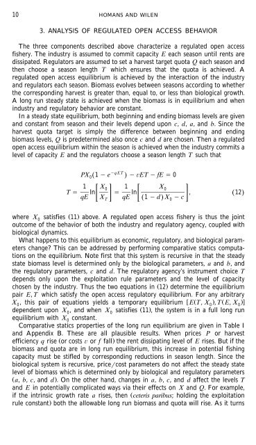
10 HOMANS AND WILEN 3. ANALYSIS OF REGULATED OPEN ACCESS BEHAVIOR The three components described above characterize a regulated open access fishery. The industry is assumed to commit capacity E each season until rents are dissipated. Regulators are assumed to set a harvest target quota Q each season and then choose a season length T which ensures that the quota is achieved. A regulated open access equilibrium is achieved by the interaction of the industry and regulators each season. Biomass evolves between seasons according to whether the corresponding harvest is greater than, equal to, or less than biological growth. A long run steady state is achieved when the biomass is in equilibrium and when industry and regulatory behavior are constant. In a steady state equilibrium, both beginning and ending biomass levels are given and constant from season and their levels depend upon c, d, a, and b. Since the harvest quota target is simply the difference between beginning and ending biomass levels, Q is predetermined also once c and d are chosen. Then a regulated open access equilibrium within the season is achieved when the industry commits a level of capacity E and the regulators choose a season length T such that PX0Ž 1 e qET . ET fE 0 1 X0 1 X0 T ln ln , Ž 12. qE X qE Ž 1 d. X c T 0 where X satisfies Ž 11. 0 above. A regulated open access fishery is thus the joint outcome of the behavior of both the industry and regulatory agency, coupled with biological dynamics. What happens to this equilibrium as economic, regulatory, and biological parameters change? This can be addressed by performing comparative statics computations on the equilibrium. Note first that this system is recursive in that the steady state biomass level is determined only by the biological parameters, a and b, and the regulatory parameters, c and d. The regulatory agency’s instrument choice T depends only upon the exploitation rule parameters and the level of capacity chosen by the industry. Thus the two equations in Ž 12. determine the equilibrium pair E, T which satisfy the open access regulatory equilibrium. For any arbitrary X , this pair of equations yields a temporary equilibrium ET,X Ž .,TŽ E, X . 0 0 0 dependent upon X , and when X satisfies Ž 11 . 0 0 , the system is in a full long run equilibrium with X0 constant. Comparative statics properties of the long run equilibrium are given in Table I and Appendix B. These are all plausible results. When prices P or harvest efficiency q rise Ž or costs or f fall. the rent dissipating level of E rises. But if the biomass and quota are in long run equilibrium, this increase in potential fishing capacity must be stifled by corresponding reductions in season length. Since the biological system is recursive, pricecost parameters do not affect the steady state level of biomass which is determined only by biological and regulatory parameters Ž a, b, c, and d .. On the other hand, changes in a, b, c, and d affect the levels T and E in potentially complicated ways via their effects on X and Q. For example, if the intrinsic growth rate a rises, then Žceteris paribus; holding the exploitation rule constant. both the allowable long run biomass and quota will rise. As it turns
REGULATED OPEN ACCESS RESOURCE USE 11 TABLE I Comparative Statics Variable E T X Q P 0 0 0 0 f 0 0 q 0 0 a b c ? ? ? d ? ? ? out, this higher quota is achieved with an increase in the equilibrium level of fishing capacity and a decrease in the regulated season length. The only ambiguous results are those associated with the effects of changes in the regulatory parameters c and d on E and T. Recall that increasing the quota rule parameter d reduces the steady state biomass level while it increases the fraction of initial biomass targeted for harvest. Thus whether or not an increase in d will attract more entry depends upon the interplay between two forces in their effects on revenues. On the one hand, a lower steady state biomass level will reduce E ceteris paribus because there is a stock effect via the production function. On the other hand, increasing the exploitation rate increases the fraction of initial biomass allowed to be taken. If d is such that the steady state biomass is to the right of X msy, then increasing d has opposing effects: a reduction in revenues via the stock effect of a reduced biomass level on the harvest function, and an increase in revenues via the fact that lower biomass levels actually increase the amount of growth and hence steady state yield. If d is relatively large, however, so that the equilibrium is to the left of X msy, increases in d cause a negative stock effect and a reduction in allowable harvest, both of which lead to lower E and longer T. The bottom line is that for large enough values of d, the derivative of E with respect to d is negative and the derivative of T with respect to d is positive, whereas for smaller values these signs are indeterminate. Note that the qualitative properties of the regulated open access model are different from those predicted by the pure open access Gordon model in fundamental ways. In the Gordon model, rents generate excess capacity, which in turn results in excessive harvest levels. These harvest levels, coupled with biological dynamics, determine an approach to a bioeconomic equilibrium. With higher prices andor lower costs, the bioeconomic equilibrium will occur at lower, more vulnerable biomass levels. In the model presented here, the existence of the regulatory structure decouples the effects of economic parameters from impacts on the biomass. To the extent that the regulatory structure is effective, the biomass level will approach its safe level. Harvest quota targets ensure this, but the manner in which they are implemented depends upon the interplay between biological and economic factors. For example, when prices are high, potential rents attract more capacity which is stifled on the grounds with short seasons so that the targeted harvest quota is not exceeded. In the long run the regulated open access fishery
Page 1 and 2: Ž . JOURNAL OF ENVIRONMENTAL ECONO
Page 3 and 4: REGULATED OPEN ACCESS RESOURCE USE
Page 9: REGULATED OPEN ACCESS RESOURCE USE
Page 21: REGULATED OPEN ACCESS RESOURCE USE

A Model of Regulated Open Access Resource Use

Create successful ePaper yourself

Delete template?

Save as template?